def finite_diff(f, x, h=1e-6):
    return (f(x+h)-f(x)) / h
Introduction
Differentiable Programming is when your code – understood as defining some mapping from inputs to outputs – can be differentiated algorithmically.
To further our understanding of complex systems like galaxies, brains, climate and society, scientific inquiry increasingly relies on computer simulations.
When models are expressed not as analytic mathematical expressions on a piece of paper, but as computer code, we still need a way to compute their derivatives. And we need it to be as efficient as possible.
This report – in conjunction with the seminar talk – aims to motivate and explain the approaches to compute gradients of code. You will get an overview of the techniques, how the details of their inner workings impact their efficiency and look at the key design principles of modern automatic differentiation frameworks as well as their practical use.
While beginning with straight forward numerical and symbolical differentiation, we cover
- the foundation of all machine learning magic, backprop, allowing efficient and automatic differentiation of neural networks, see Section 4
- the differentiable future of simulation, source-to-source transformation for auto-differentiating arbitrary source code, see Section 5.3.
The definition of a derivative is simple and well-known:
\[ f'(x) = \lim_{h\to0}\frac{f(x+h)-f(x)}{h} \tag{1}\]
As it is that straight-forward, it directly leads to the first approach:
Finite Differences
Taking Equation 1 literally, we can choose an \(h\) that is not actually zero, but small enough to provide a close approximation to the derivative. The implementation is really simple, making this approach easily available in any language:
Unfortunately, finite differences is inefficient, as one additional forward pass is required for every variable we need to obtain the derivative for. Additionally, it can be quite imprecise and we don’t obtain an information about the quality of the approximation. There exist several refinements of the method, but the core problems persist, so we head straight to the next technique, which offers derivatives down to machine precision.
Symbolic Differentiation
If you think about the way you learned to take derivatives, finite differences probably weren’t part of that experience. That’s no wonder, as we usually get taught to take derivatives analytically. Calculating the derivative of a differentiable function from an analytic expression can be tedious, but it is a process which follows a strict set of rules. Instead of applying those rules by hand, symbolic differentiation implements them in computer code. Unsurprisingly, this is a bit harder than the implementation of finite differences. Fortunately, libraries are available which hide the implementational details. As this isn’t our final destination yet, we will do the same and just show how SymPy can be used for symbolic differentiation in Python.
Consider the function
\[ y = \sin(2x)+x^2. \]
It can be decomposed into a computational graph (Figure 2), which contains the most basic operations and the way they are put together
Code
\definecolor{mygreen}{HTML}{d6f4c0}
\definecolor{mypink}{HTML}{ffc6c4}

\usetikzlibrary{positioning,graphs,quotes}
\tikzstyle{comp} = [draw, rectangle, rounded corners]

\tikzstyle{m} = [draw, circle, minimum size=0.6cm, inner xsep=0mm, inner ysep=0mm]
\tikzstyle{inp} = [m, fill=mygreen]
\tikzstyle{outp} = [m, fill=mypink]
{\begin{tikzpicture}
    \node[inp] (x) at (0,0) {$x$};
    \node[comp] (mult) at (-1, -1) {$2\times\cdot$};
    \node[comp] (sin) at (-1, -2) {$\sin(\cdot)$};
    \node[comp] (square) at (1, -1) {$(\cdot)^2$};
    \node[comp] (plus) at (0,-3) {$\cdot+\cdot$};
    \node[outp] (y) at (0,-4) {$y$};
    \draw[->] (x) -- (mult);
    \draw[->] (mult) -- (sin);
    \draw[->] (sin) -- (plus);
    \draw[->] (x) -- (square);
    \draw[->] (square) -- (plus);
    \draw[->] (plus) -- (y);
\end{tikzpicture}
SymPy does this (or a similar) decomposition automatically. For this to happen, we have to define our variables as symbols and use SymPy’s sine function. Addition, multiplication and power work by the use of operator overloading – SymPy defines custom functions that are used when the operation is applied to a symbol. This enables it to trace those operations and build the computational graph.
import sympy

# define symbols
x = sympy.symbols('x')

# define function
def f(x):
    return sympy.sin(2*x) + x**2

f(x)
x**2 + sin(2*x)Next, we can call sympy.diff to obtain an analytic expression of the derivative of f with respect to x.
sympy.diff(f(x), x)2*x + 2*cos(2*x)Having obtained this expression, we can now plug in any value for \(x\) and obtain the exact result, at least as exact as the computer can get (i.e., machine precision). This is great! Unfortunately though, this can not solve all of our problems. For one, the analytical expressions for the derivatives can grow very large when functions are stacked. Below, we see a simplified example for this, where we stack multiple sigmoid functions.
def sigmoid(x):
    return 1 / (1 + sympy.exp(-x))
sympy.diff(sigmoid(x), x)
exp(-x)/(1 + exp(-x))**2sympy.diff(sigmoid(sigmoid(x)), x)exp(-x)*exp(-1/(1 + exp(-x)))/((1 + exp(-x))**2*(1 + exp(-1/(1 + exp(-x))))**2)sympy.diff(sigmoid(sigmoid(sigmoid(x))), x)exp(-x)*exp(-1/(1 + exp(-x)))*exp(-1/(1 + exp(-1/(1 + exp(-x)))))/((1 + exp(-x))**2*(1 + exp(-1/(1 + exp(-x))))**2*(1 + exp(-1/(1 + exp(-1/(1 + exp(-x))))))**2)This is called expression swell and can lead to high demands with respect to memory. Additionally, most computer programs and simulators can’t be expressed as a simple differentiable expression, but contain more or less complex dynamic control flow, discontinuities and other properties that are hard to account for in symbolic differentiation. What we need is a framework that overcomes this limitations, but still provides gradients down to machine precision. That’s where automatic differentiation comes in.
Automatic Differentiation
The following discussion is strongly inspired by this talk by Matthew J Johnson, which we want to recommend to anyone who wants to know more about both the basics and the implementional details of automatic differentiation.
Basics: The univariate case
For simplicity, we will discuss the basic concepts of automatic differentiation in the univariate case first. For a multivariate discussion, see Johnson (2017). Consider the function
\[ F=D\circ C\circ B\circ A \]
\[ y=F(x)=D(C(B(A(x)))) \]
As we later want to use differentials, we also define the intermediate values
\[ a=A(x),b=B(a),c=C(b),y=d=D(c). \]
The derivative of \(y\) with respect to \(x\) is then defined by
\[ F'(x)=\frac{\partial y}{\partial x}=\frac{\partial y}{\partial d}\frac{\partial d}{\partial c}\frac{\partial c}{\partial b}\frac{\partial b}{\partial a}\frac{\partial a}{\partial x}. \]
In practice, we have some freedom when we want to calculate the derivative from the partial derivatives. As the product is associative, we can choose in which order we want to calculate the products. For reasons that will become clear later on, two main modes have emerged. In the forward mode, the product is evaluated from right to left, starting at the input and ending at the output (forward):
\[ \frac{\partial y}{\partial x}=\frac{\partial y}{\partial d}\left(\frac{\partial d}{\partial c}\left(\frac{\partial c}{\partial b}\left(\frac{\partial b}{\partial a}\frac{\partial a}{\partial x}\right)\right)\right) \]
In reverse mode, the process is reversed, starting at the output and moving towards the input:
\[ \frac{\partial y}{\partial x}=\left(\left(\left(\frac{\partial y}{\partial d}\frac{\partial d}{\partial c}\right)\frac{\partial c}{\partial b}\right)\frac{\partial b}{\partial a}\right)\frac{\partial a}{\partial x} \]
Note that the result will be exactly the same, only the order of the multiplications changed.
Automatic differentiation as message passing
Using the computational graph, we can see that automatic differentiation can be thought of as message passing along the graph. The mode determines in which direction the messages go.
In forward mode, we initialize the differentials at the input. Moving through the graph, each node collects the differentials of all its parents (so that no relevant information is lost). This can be formalized into the rule
\[ \delta_j=\sum_{k\in\text{parents}(j)}\frac{\partial j}{\partial k}\delta_k. \tag{2}\]
In the univariate case, each node only has one parent, but this formulation naturally generalizes to the multivariate case (see below). If we initialize with \(\delta_x=1\), we can see that the complete derivative can be collected at the output.
Code
\definecolor{mygreen}{HTML}{d6f4c0}
\definecolor{mypink}{HTML}{ffc6c4}
\definecolor{mygrey}{HTML}{dddddd}
\definecolor{mylightgreen}{HTML}{eeffee}
\definecolor{myred}{HTML}{ffeeee}
\definecolor{dcol}{HTML}{223399}

\usetikzlibrary{positioning,graphs,quotes}
\tikzstyle{comp} = [draw, rectangle, rounded corners]

\tikzstyle{m} = [draw, circle, minimum size=0.6cm, inner xsep=0mm, inner ysep=0mm]
\tikzstyle{inp} = [m, fill=mygreen]
\tikzstyle{outp} = [m, fill=mypink]
\tikzstyle{op} = [m, fill=mygrey]
\tikzstyle{dl} = [draw, circle, dotted, fill=mylightgreen, minimum size=0.55cm, xshift=-0.1cm,font=\small,inner ysep=0, inner xsep=0, text=dcol]
\tikzstyle{dt} = [dl,xshift=0.1cm]
\tikzstyle{dr} = [dl, fill=myred]
\tikzstyle{eq} = [font=\small,align=center]
\tikzstyle{eqr} = [eq,xshift=-0.1cm]
\tikzstyle{eql} = [eq,xshift=0.1cm]
\tikzstyle{diff} = [->, dotted,swap,font=\footnotesize, inner xsep=0.5mm, inner ysep=0.1mm, text=dcol, dcol]
\tikzstyle{dval} = [font=\footnotesize,xshift=0.38cm,text=dcol]
\tikzstyle{dtval} = [font=\footnotesize,xshift=-0.35cm,text=dcol]

\begin{tikzpicture}[thick]
            \node[inp] (x) at (0,0) {$x$};
            \node[op,yshift=-0.4cm] (a) at (1.8,0) {$A$};
            \node[op] (b) at (3.6,0) {$B$};
            \node[op,yshift=-0.4cm] (c) at (5.4,0) {$C$};
            \node[op] (d) at (7.2,0) {$D$};
            \node[outp,yshift=-0.4cm] (y) at (9.0,0) {$y$};

            \draw[->] (x) -- (a);
            \draw[->] (a) -- (b);
            \draw[->] (b) -- (c);
            \draw[->] (c) -- (d);
            \draw[->] (d) -- (y);

            \draw (x.330) edge[diff,"$\delta_x$"] (a.185);
            \draw (a.355) edge[diff,"$\delta_a$"] (b.210);
            \draw (b.330) edge[diff,"$\delta_b$"] (c.185);
            \draw (c.355) edge[diff,"$\delta_c$"] (d.210);
            \draw (d.330) edge[diff,"$\delta_d$"] (y.185);

            \node[above of=x,yshift=-0.3cm,align=center,font=\small] (dx) {$\delta_x=\frac{\partial x}{\partial x}$\\$=1$};
            \node[below of=a,yshift=0.3cm,align=center,font=\small] (da) {$\delta_a=\frac{\partial a}{\partial x}\delta_x$};
            \node[above of=b,yshift=-0.17cm,align=center,font=\small] (db) {$\delta_b=\frac{\partial b}{\partial a}\delta_a$\\$=\frac{\partial b}{\partial a}\frac{\partial a}{\partial x}\delta_x$};
            \node[below of=c,yshift=0.17cm,align=center,font=\small] (dc) {$\delta_c=\frac{\partial c}{\partial b}\delta_b$\\$=\frac{\partial c}{\partial b}\frac{\partial b}{\partial a}\frac{\partial a}{\partial x}\delta_x$};
            \node[above of=d,yshift=-0.17cm,align=center,font=\small] (dd) {$\delta_d=\frac{\partial d}{\partial c}\delta_c$\\$=\frac{\partial d}{\partial c}\frac{\partial c}{\partial b}\frac{\partial b}{\partial a}\frac{\partial a}{\partial x}\delta_x$};
            \node[below of=y,yshift=-0.1cm,align=center,font=\small] (dy) {$\delta_y=\frac{\partial y}{\partial d}\delta_d$\\$=\frac{\partial y}{\partial d}\frac{\partial d}{\partial c}\frac{\partial c}{\partial b}\frac{\partial b}{\partial a}\frac{\partial a}{\partial x}\delta_x$\\$=\frac{\partial y}{\partial x}\delta_x=\frac{\partial y}{\partial x}$};

        \end{tikzpicture}
In reverse mode, we initialize the differential at the output. Next, each node collects the derivatives of all its children (again, this is necessary to make sure no information is lost):
\[ \bar\delta_k=\sum_{j\in\text{children}(k)}\bar\delta_j\frac{\partial j}{\partial k} \tag{3}\]
Figure 4 shows the process for the univariate case. In reverse mode, the complete derivative ends up at the input node. Even in reverse mode, we might need information on the intermediate values of \(a, b, c, ...\) to compute the partial derivatives, so one forward pass (indicated by the arrows with solid lines) is necessary before the backward pass can be conducted.
Code
\definecolor{mygreen}{HTML}{d6f4c0}
\definecolor{mypink}{HTML}{ffc6c4}
\definecolor{mygrey}{HTML}{dddddd}
\definecolor{mylightgreen}{HTML}{eeffee}
\definecolor{myred}{HTML}{ffeeee}
\definecolor{dcol}{HTML}{223399}

\usetikzlibrary{positioning,graphs,quotes}
\tikzstyle{comp} = [draw, rectangle, rounded corners]

\tikzstyle{m} = [draw, circle, minimum size=0.6cm, inner xsep=0mm, inner ysep=0mm]
\tikzstyle{inp} = [m, fill=mygreen]
\tikzstyle{outp} = [m, fill=mypink]
\tikzstyle{op} = [m, fill=mygrey]
\tikzstyle{dl} = [draw, circle, dotted, fill=mylightgreen, minimum size=0.55cm, xshift=-0.1cm,font=\small,inner ysep=0, inner xsep=0, text=dcol]
\tikzstyle{dt} = [dl,xshift=0.1cm]
\tikzstyle{dr} = [dl, fill=myred]
\tikzstyle{eq} = [font=\small,align=center]
\tikzstyle{eqr} = [eq,xshift=-0.1cm]
\tikzstyle{eql} = [eq,xshift=0.1cm]
\tikzstyle{diff} = [<-, dotted,swap,font=\footnotesize, inner xsep=0.5mm, inner ysep=0.1mm, text=dcol, dcol]
\tikzstyle{dval} = [font=\footnotesize,xshift=0.38cm,text=dcol]
\tikzstyle{dtval} = [font=\footnotesize,xshift=-0.35cm,text=dcol]


\begin{tikzpicture}[thick]
            \node[inp] (x) at (0,0) {$x$};
            \node[op,yshift=-0.4cm] (a) at (1.8,0) {$A$};
            \node[op] (b) at (3.6,0) {$B$};
            \node[op,yshift=-0.4cm] (c) at (5.4,0) {$C$};
            \node[op] (d) at (7.2,0) {$D$};
            \node[outp,yshift=-0.4cm] (y) at (9.0,0) {$y$};

            \draw[->] (x) -- (a);
            \draw[->] (a) -- (b);
            \draw[->] (b) -- (c);
            \draw[->] (c) -- (d);
            \draw[->] (d) -- (y);

            \draw (x.330) edge[diff,"$\bar\delta_a$"] (a.185);
            \draw (a.355) edge[diff,"$\bar\delta_b$"] (b.210);
            \draw (b.330) edge[diff,"$\bar\delta_c$"] (c.185);
            \draw (c.355) edge[diff,"$\bar\delta_d$"] (d.210);
            \draw (d.330) edge[diff,"$\bar\delta_y$"] (y.185);

            \node[above of=x,yshift=0.1cm,align=center,font=\small] (dx) {$\bar\delta_x=\bar\delta_a\frac{\partial a}{\partial x}$\\$=\bar\delta_y\frac{\partial y}{\partial d}\frac{\partial d}{\partial c}\frac{\partial c}{\partial b}\frac{\partial b}{\partial a}\frac{\partial a}{\partial x}$\\$=\bar\delta_y\frac{\partial y}{\partial x}=\frac{\partial y}{\partial x}$};
            \node[below of=a,yshift=0.17cm,align=center,font=\small] (da) {$\bar\delta_a=\bar\delta_b\frac{\partial b}{\partial a}$\\$=\bar\delta_y\frac{\partial y}{\partial d}\frac{\partial d}{\partial c}\frac{\partial c}{\partial b}\frac{\partial b}{\partial a}$};
            \node[above of=b,yshift=-0.17cm,align=center,font=\small] (db) {$\bar\delta_b=\bar\delta_c\frac{\partial c}{\partial b}$\\$=\bar\delta_y\frac{\partial y}{\partial d}\frac{\partial d}{\partial c}\frac{\partial c}{\partial b}$};
            \node[below of=c,yshift=0.17cm,align=center,font=\small] (dc) {$\bar\delta_c=\bar\delta_d\frac{\partial d}{\partial c}$\\$=\bar\delta_y\frac{\partial y}{\partial d}\frac{\partial d}{\partial c}$};
            \node[above of=d,yshift=-0.17cm,align=center,font=\small] (dd) {$\bar\delta_d=\bar\delta_y\frac{\partial y}{\partial d}$};
            \node[below of=y,yshift=-0.1cm,align=center,font=\small] (dy) {$\bar\delta_y=\frac{\partial y}{\partial y}$\\$=1$};

        \end{tikzpicture}
Note that the differentials \(\delta_k\) in forward mode and \(\bar\delta_k\) in reverse mode differ. The first contains the information from its ancestors, whereas the latter contains the information from its children.
A multivariate example
The above discussion of the univariate case served to explain the core ideas, but the distinction between forward and reverse mode only becomes relevant in the multivariate case. We will explore the main concepts using a simple, low-dimensional example. Consider the function \(f: \mathbb{R}^3\to\mathbb{R}^2\) with
\[ (x,w,b) \mapsto \begin{pmatrix} y_1 \\ y_2 \end{pmatrix}=\begin{pmatrix} (xw)^2 \\ xw+b \end{pmatrix}. \] Our goal is to obtain the full Jacobian matrix, which generalizes the derivative to multivariate functions:
\[ J_f = \begin{pmatrix} \frac{\partial y_1}{\partial x} & \frac{\partial y_1}{\partial w} & \frac{\partial y_1}{\partial b} \\ \frac{\partial y_2}{\partial x} & \frac{\partial y_2}{\partial w} & \frac{\partial y_2}{\partial b} \end{pmatrix} \] First, we can translate this function into a computational graph:
Code
\definecolor{mygreen}{HTML}{d6f4c0}
\definecolor{mypink}{HTML}{ffc6c4}
\definecolor{mygrey}{HTML}{dddddd}
\definecolor{mylightgreen}{HTML}{eeffee}
\definecolor{myred}{HTML}{ffeeee}
\definecolor{dcol}{HTML}{223399}

\usetikzlibrary{positioning,graphdrawing,graphs,quotes}
\usegdlibrary{layered}
\tikzstyle{comp} = [draw, rectangle, rounded corners]

\tikzstyle{m} = [draw, circle, minimum size=0.6cm, inner xsep=0mm, inner ysep=0mm]
\tikzstyle{inp} = [m, fill=mygreen]
\tikzstyle{outp} = [m, fill=mypink]
\tikzstyle{op} = [m, fill=mygrey]
\tikzstyle{dl} = [draw, circle, dotted, fill=mylightgreen, minimum size=0.55cm, xshift=-0.1cm,font=\small,inner ysep=0, inner xsep=0, text=dcol]
\tikzstyle{dt} = [dl,xshift=0.1cm]
\tikzstyle{dr} = [dl, fill=myred]
\tikzstyle{eq} = [font=\small,align=center]
\tikzstyle{eqr} = [eq,xshift=-0.1cm]
\tikzstyle{eql} = [eq,xshift=0.1cm]
\tikzstyle{diff} = [->, dotted,swap,font=\footnotesize, inner xsep=0.5mm, inner ysep=0.1mm, text=dcol, dcol]
\tikzstyle{dval} = [font=\footnotesize,xshift=0.38cm,text=dcol]
\tikzstyle{dtval} = [font=\footnotesize,xshift=-0.35cm,text=dcol]

\newcounter{x}
\newcounter{w}
\newcounter{b}
\newcounter{u}
\newcounter{vone}
\newcounter{vtwo}

\newcounter{dx}
\newcounter{dw}
\newcounter{db}
\newcounter{du}
\newcounter{dvone}
\newcounter{dvtwo}
\newcounter{dyone}
\newcounter{dytwo}

\setcounter{x}{3}
\setcounter{w}{2}
\setcounter{b}{1}

        \begin{tikzpicture}[thick]
            \setcounter{u}{\numexpr \thex * \thew \relax}
            \setcounter{vone}{\numexpr \theu * \theu \relax}
            \setcounter{vtwo}{\numexpr \theb + \theu \relax}

            \setcounter{du}{\numexpr \thew * \thedx + \thex * \thedw \relax}
            \setcounter{dvone}{\numexpr \thedu * 2 * \theu \relax}
            \setcounter{dvtwo}{\numexpr \thedu + \thedb \relax}
            \setcounter{dyone}{\thedvone}
            \setcounter{dytwo}{\thedvtwo}
            \graph[layered layout, grow=down, nodes={draw, circle}, sibling distance=3.8cm, level distance=2cm] {
                { [same layer] x[inp, as={$\cdot$}], w[inp, as={$\cdot$}], b[inp, as={$\cdot$}] };
                { [same layer] prod[op,as=$\times$, xshift=-1.8cm] };
                { [same layer] v2[op, as=$+$], v1[op, as=\small$()^2$, xshift=-1.8cm]};
                { [same layer] y1[outp, as={$\cdot$}, xshift=-1.8cm], y2[outp, as={$\cdot$}] };


                {b, prod} -> v2 -> y2;
                prod -> v1 -> y1;
                {x, w} -> prod;

            };
            % Values of inputs
            \node [right of=x,eqr](xval) {$x=\thex$};
            \node [right of=w,eqr](wval) {$w=\thew$};
            \node [right of=b,eqr](bval) {$b=\theb$};
            % product
            \node [right of=prod,eqr,,xshift=0.2cm](prodval) {$u=xw$};
            \node [right of=v1,eqr,xshift=0.3cm](v1val) {$v_1=u^2$};
            \node [right of=v2,eqr,xshift=0.5cm](v2val) {$v_2=u+b$};
            % Outputs
            \node [right of=y1,eqr,xshift=0.3cm](y1val) {$y_1=v_1$};
            \node [right of=y2,eqr,xshift=0.3cm](y2val) {$y_2=v_2$};


            \node[xshift=1.5cm,yshift=-2.6cm,scale=0.9] at (current page.south west){%
                $%
                J_f = %
                \begin{pmatrix}%
                    ? & ? & ? \\%
                    ? & ? & ?%
                \end{pmatrix}$};
        \end{tikzpicture}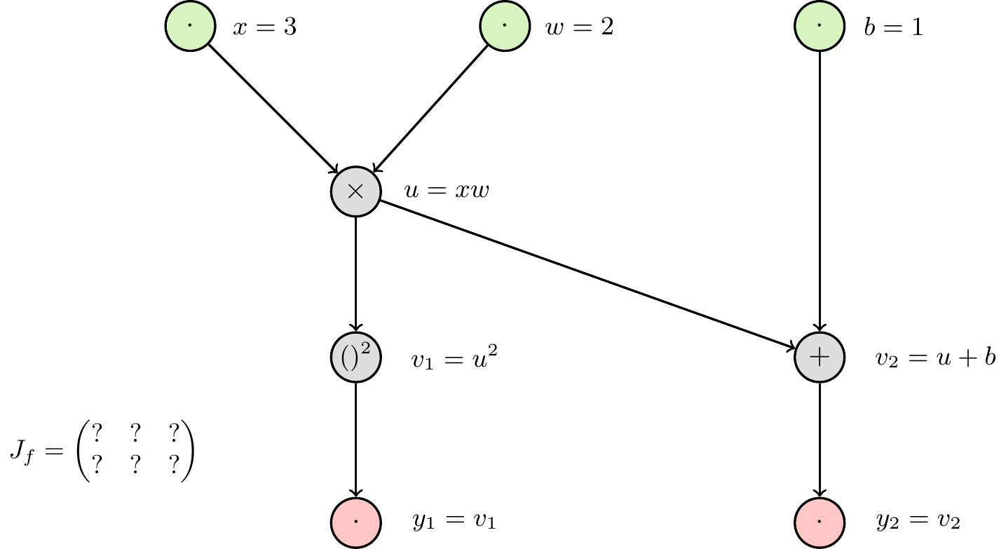
Forward mode
Using Equation 2, we can determine the way the differentials are passed through the graph (Figure 6). The partial derivatives at each node are easy to calculate (see Figure 7).
How can we make use of this graph to obtain the Jacobian matrix? We saw above that initializing the differentials at the input with 1 allowed us to read off the complete partial derivative at the output. If we did this with all differentials, setting \(\delta_x=\delta_w=\delta_b=1\), we would obtain the sum of the partial derivatives of \(\boldsymbol{y}\) with respect to \(x\), \(w\) and \(b\). As we are interested in the partial derivatives w.r.t each input, we eleminate the influence of the others by initializing the respective differentials with 0. Thereby, we can obtain one column of the Jacobian in each pass through the network. As a consequence, we have to make as many passes as there are inputs (here: three) to obtain the complete Jacobian matrix. See Figure 8 to Figure 10 for a detailed depiction of each pass.
Typically, calculating and passing the differentials has similar complexity as calculating the forward pass itself. As the function value is needed to calculate the derivative, we calculate them jointly and obtain the function value as a “side product” of the automatic differentiation.
Code
\definecolor{mygreen}{HTML}{d6f4c0}
\definecolor{mypink}{HTML}{ffc6c4}
\definecolor{mygrey}{HTML}{dddddd}
\definecolor{mylightgreen}{HTML}{eeffee}
\definecolor{myred}{HTML}{ffeeee}
\definecolor{dcol}{HTML}{223399}

\usetikzlibrary{positioning,graphdrawing,graphs,quotes}
\usegdlibrary{layered}
\tikzstyle{comp} = [draw, rectangle, rounded corners]

\tikzstyle{m} = [draw, circle, minimum size=0.6cm, inner xsep=0mm, inner ysep=0mm]
\tikzstyle{inp} = [m, fill=mygreen]
\tikzstyle{outp} = [m, fill=mypink]
\tikzstyle{op} = [m, fill=mygrey]
\tikzstyle{dl} = [draw, circle, dotted, fill=mylightgreen, minimum size=0.55cm, xshift=-0.1cm,font=\small,inner ysep=0, inner xsep=0, text=dcol]
\tikzstyle{dt} = [dl,xshift=0.1cm]
\tikzstyle{dr} = [dl, fill=myred]
\tikzstyle{eq} = [font=\small,align=center]
\tikzstyle{eqr} = [eq,xshift=-0.1cm]
\tikzstyle{eql} = [eq,xshift=0.1cm]
\tikzstyle{diff} = [->, dotted,swap,font=\footnotesize, inner xsep=0.5mm, inner ysep=0.1mm, text=dcol, dcol]
\tikzstyle{dval} = [font=\footnotesize,xshift=0.38cm,text=dcol]
\tikzstyle{dtval} = [font=\footnotesize,xshift=-0.35cm,text=dcol]

\newcounter{x}
\newcounter{w}
\newcounter{b}
\newcounter{u}
\newcounter{vone}
\newcounter{vtwo}

\newcounter{dx}
\newcounter{dw}
\newcounter{db}
\newcounter{du}
\newcounter{dvone}
\newcounter{dvtwo}
\newcounter{dyone}
\newcounter{dytwo}

\setcounter{x}{3}
\setcounter{w}{2}
\setcounter{b}{1}

\begin{tikzpicture}[thick]
    \setcounter{u}{\numexpr \thex * \thew \relax}
    \setcounter{vone}{\numexpr \theu * \theu \relax}
    \setcounter{vtwo}{\numexpr \theb + \theu \relax}

    \setcounter{du}{\numexpr \thew * \thedx + \thex * \thedw \relax}
    \setcounter{dvone}{\numexpr \thedu * 2 * \theu \relax}
    \setcounter{dvtwo}{\numexpr \thedu + \thedb \relax}
    \setcounter{dyone}{\thedvone}
    \setcounter{dytwo}{\thedvtwo}
    \graph[layered layout, grow=down, nodes={draw, circle}, sibling distance=3.8cm, level distance=2cm] {
        { [same layer] x[inp, as={$\cdot$}], w[inp, as={$\cdot$}], b[inp, as={$\cdot$}] };
        { [same layer] prod[op,as=$\times$, xshift=-1.8cm] };
        { [same layer] v2[op, as=$+$], v1[op, as=\small$()^2$, xshift=-1.8cm]};
        { [same layer] y1[outp, as={$\cdot$}, xshift=-1.8cm], y2[outp, as={$\cdot$}] };


        {b, prod} -> v2 -> y2;
        prod -> v1 -> y1;
        {x, w} -> prod;

    };
    % Input differentials
    \node [left of=x,dl](dx) {$\delta_x$};
    \node [left of=dx,dval](dxval) {};
    \draw[diff] (dx) -- (x);
    \node [left of=w,dl](dw) {$\delta_w$};
    \node [left of=dw,dval](dwval) {};
    \draw[diff] (dw) -- (w);
    \node [left of=b,dl](db) {$\delta_b$};
    \node [left of=db,dval](dbval) {};
    \draw[diff] (db) -- (b);
    % Values of inputs
    \node [right of=x,eqr](xval) {$x=\thex$};
    \node [right of=w,eqr](wval) {$w=\thew$};
    \node [right of=b,eqr](bval) {$b=\theb$};
    % product
    \node [right of=prod,eqr](prodval) {$u=xw$};
    \node [left of=prod,eql,align=center,xshift=-0.9cm](du) {$\color{dcol}\delta_u\color{black}=\frac{\partial u}{\partial x}\color{dcol}\delta_x\color{black}+\frac{\partial u}{\partial w}\color{dcol}\delta_w$};
    % v1
    \node [right of=v1,eqr,xshift=0.1cm](v1val) {$v_1=u^2$};
    \node [left of=v1,eql,xshift=-0.5cm](dyone) {$\color{dcol}\delta_{v_1}\color{black}=\frac{\partial v_1}{\partial u}\cdot\color{dcol}\delta_u$};
    % v2
    \node [right of=v2,eqr,xshift=0.25cm](v2val) {$v_2=u+b$};
    \node [left of=v2,eql,xshift=-0.92cm,yshift=-0.1cm](dytwo) {$\color{dcol}\delta_{v_2}\color{black}=\frac{\partial v_2}{\partial u}\color{dcol}\delta_u\color{black}+\frac{\partial v_2}{\partial b}\color{dcol}\delta_b$};
    % Outputs
    \node [left of=y1,dr](dy1) {$\delta_{y_1}$};
    \node [right of=y1,eqr,xshift=0.1cm](y1val) {$y_1=v_1$};
    \draw[diff] (y1) -- (dy1);
    \node [left of=dy1,dval](dy1val) {};
    \node [left of=y2,dr](dy2) {$\delta_{y_2}$};
    \node [right of=y2,eqr](y2val) {$y_2=v_2$};
    \draw[diff] (y2) -- (dy2);
    \node [left of=dy2,dval](dy2val) {};

    % Path of differentials
    \draw (x.300) edge[diff,"$\delta_x$"] (prod.155);
    \draw (prod.250) edge[diff,"$\delta_u$"] (v1.110);
    \draw (v1.250) edge[diff,"$\delta_{v_1}$"] (y1.110);
    \draw (w.205) edge[diff,"$\delta_w$"] (prod.65);
    \draw (b.250) edge[diff,"$\delta_b$"] (v2.110);
    \draw (v2.250) edge[diff,"$\delta_{v_2}$"] (y2.110);
    \draw (prod.325) edge[diff,"$\delta_u$"] (v2.175);

    \node[xshift=1.5cm,yshift=-2.6cm,scale=0.9] at (current page.south west){%
        $%
        J_f = %
        \begin{pmatrix}%
            ? & ? & ? \\%
            ? & ? & ?%
        \end{pmatrix}$};
\end{tikzpicture}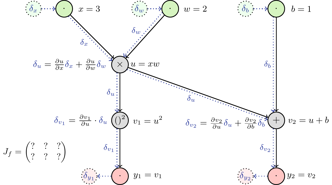
Code
\definecolor{mygreen}{HTML}{d6f4c0}
\definecolor{mypink}{HTML}{ffc6c4}
\definecolor{mygrey}{HTML}{dddddd}
\definecolor{mylightgreen}{HTML}{eeffee}
\definecolor{myred}{HTML}{ffeeee}
\definecolor{dcol}{HTML}{223399}

\usetikzlibrary{positioning,graphdrawing,graphs,quotes}
\usegdlibrary{layered}
\tikzstyle{comp} = [draw, rectangle, rounded corners]

\tikzstyle{m} = [draw, circle, minimum size=0.6cm, inner xsep=0mm, inner ysep=0mm]
\tikzstyle{inp} = [m, fill=mygreen]
\tikzstyle{outp} = [m, fill=mypink]
\tikzstyle{op} = [m, fill=mygrey]
\tikzstyle{dl} = [draw, circle, dotted, fill=mylightgreen, minimum size=0.55cm, xshift=-0.1cm,font=\small,inner ysep=0, inner xsep=0, text=dcol]
\tikzstyle{dt} = [dl,xshift=0.1cm]
\tikzstyle{dr} = [dl, fill=myred]
\tikzstyle{eq} = [font=\small,align=center]
\tikzstyle{eqr} = [eq,xshift=-0.1cm]
\tikzstyle{eql} = [eq,xshift=0.1cm]
\tikzstyle{diff} = [->, dotted,swap,font=\footnotesize, inner xsep=0.5mm, inner ysep=0.1mm, text=dcol, dcol]
\tikzstyle{dval} = [font=\footnotesize,xshift=0.38cm,text=dcol]
\tikzstyle{dtval} = [font=\footnotesize,xshift=-0.35cm,text=dcol]

\newcounter{x}
\newcounter{w}
\newcounter{b}
\newcounter{u}
\newcounter{vone}
\newcounter{vtwo}

\newcounter{dx}
\newcounter{dw}
\newcounter{db}
\newcounter{du}
\newcounter{dvone}
\newcounter{dvtwo}
\newcounter{dyone}
\newcounter{dytwo}

\setcounter{x}{3}
\setcounter{w}{2}
\setcounter{b}{1}

\begin{tikzpicture}[thick]
    \setcounter{u}{\numexpr \thex * \thew \relax}
    \setcounter{vone}{\numexpr \theu * \theu \relax}
    \setcounter{vtwo}{\numexpr \theb + \theu \relax}

    \setcounter{du}{\numexpr \thew * \thedx + \thex * \thedw \relax}
    \setcounter{dvone}{\numexpr \thedu * 2 * \theu \relax}
    \setcounter{dvtwo}{\numexpr \thedu + \thedb \relax}
    \setcounter{dyone}{\thedvone}
    \setcounter{dytwo}{\thedvtwo}
    \graph[layered layout, grow=down, nodes={draw, circle}, sibling distance=3.8cm, level distance=2cm] {
        { [same layer] x[inp, as={$\cdot$}], w[inp, as={$\cdot$}], b[inp, as={$\cdot$}] };
        { [same layer] prod[op,as=$\times$, xshift=-1.8cm] };
        { [same layer] v2[op, as=$+$], v1[op, as=\small$()^2$, xshift=-1.8cm]};
        { [same layer] y1[outp, as={$\cdot$}, xshift=-1.8cm], y2[outp, as={$\cdot$}] };


        {b, prod} -> v2 -> y2;
        prod -> v1 -> y1;
        {x, w} -> prod;

    };
    % Input differentials
    \node [left of=x,dl](dx) {$\delta_x$};
    \node [left of=dx,dval](dxval) {};
    \draw[diff] (dx) -- (x);
    \node [left of=w,dl](dw) {$\delta_w$};
    \node [left of=dw,dval](dwval) {};
    \draw[diff] (dw) -- (w);
    \node [left of=b,dl](db) {$\delta_b$};
    \node [left of=db,dval](dbval) {};
    \draw[diff] (db) -- (b);
    % Values of inputs
    \node [right of=x,eqr](xval) {$x=\thex$};
    \node [right of=w,eqr](wval) {$w=\thew$};
    \node [right of=b,eqr](bval) {$b=\theb$};
    % product
    \node [right of=prod,eqr](prodval) {$u=xw$};
    \node [left of=prod,eql,align=center,xshift=-0.9cm](du) {$\color{dcol}\delta_u\color{black}=w\color{dcol}\delta_x\color{black}+x\color{dcol}\delta_w$};
    % v1
    \node [right of=v1,eqr,xshift=0.1cm](v1val) {$v_1=u^2$};
    \node [left of=v1,eql,xshift=-0.5cm](dyone) {$\color{dcol}\delta_{v_1}\color{black}=2u\cdot\color{dcol}\delta_u$};
    % v2
    \node [right of=v2,eqr,xshift=0.25cm](v2val) {$v_2=u+b$};
    \node [left of=v2,eql,xshift=-0.92cm,yshift=-0.1cm](dytwo) {$\color{dcol}\delta_{v_2}\color{black}=1\cdot\color{dcol}\delta_u\color{black}+1\cdot\color{dcol}\delta_b$};
    % Outputs
    \node [left of=y1,dr](dy1) {$\delta_{y_1}$};
    \node [right of=y1,eqr,xshift=0.1cm](y1val) {$y_1=v_1$};
    \draw[diff] (y1) -- (dy1);
    \node [left of=dy1,dval](dy1val) {};
    \node [left of=y2,dr](dy2) {$\delta_{y_2}$};
    \node [right of=y2,eqr](y2val) {$y_2=v_2$};
    \draw[diff] (y2) -- (dy2);
    \node [left of=dy2,dval](dy2val) {};

    % Path of differentials
    \draw (x.300) edge[diff,"$\delta_x$"] (prod.155);
    \draw (prod.250) edge[diff,"$\delta_u$"] (v1.110);
    \draw (v1.250) edge[diff,"$\delta_{v_1}$"] (y1.110);
    \draw (w.205) edge[diff,"$\delta_w$"] (prod.65);
    \draw (b.250) edge[diff,"$\delta_b$"] (v2.110);
    \draw (v2.250) edge[diff,"$\delta_{v_2}$"] (y2.110);
    \draw (prod.325) edge[diff,"$\delta_u$"] (v2.175);

    \node[xshift=1.5cm,yshift=-2.6cm,scale=0.9] at (current page.south west){%
        $%
        J_f = %
        \begin{pmatrix}%
            ? & ? & ? \\%
            ? & ? & ?%
        \end{pmatrix}$};
\end{tikzpicture}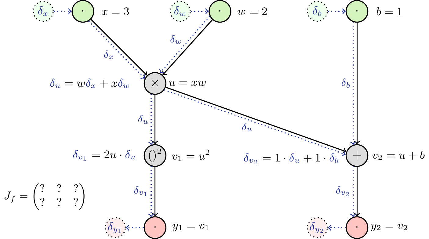
Code
\definecolor{mygreen}{HTML}{d6f4c0}
\definecolor{mypink}{HTML}{ffc6c4}
\definecolor{mygrey}{HTML}{dddddd}
\definecolor{mylightgreen}{HTML}{eeffee}
\definecolor{myred}{HTML}{ffeeee}
\definecolor{dcol}{HTML}{223399}
\definecolor{BrickRed}{rgb}{0.8, 0.25, 0.33}

\usetikzlibrary{positioning,graphdrawing,graphs,quotes}
\usegdlibrary{layered}
\tikzstyle{comp} = [draw, rectangle, rounded corners]

\tikzstyle{m} = [draw, circle, minimum size=0.6cm, inner xsep=0mm, inner ysep=0mm]
\tikzstyle{inp} = [m, fill=mygreen]
\tikzstyle{outp} = [m, fill=mypink]
\tikzstyle{op} = [m, fill=mygrey]
\tikzstyle{dl} = [draw, circle, dotted, fill=mylightgreen, minimum size=0.55cm, xshift=-0.1cm,font=\small,inner ysep=0, inner xsep=0, text=dcol]
\tikzstyle{dt} = [dl,xshift=0.1cm]
\tikzstyle{dr} = [dl, fill=myred]
\tikzstyle{eq} = [font=\small,align=center]
\tikzstyle{eqr} = [eq,xshift=-0.1cm]
\tikzstyle{eql} = [eq,xshift=0.1cm]
\tikzstyle{diff} = [->, dotted,swap,font=\footnotesize, inner xsep=0.5mm, inner ysep=0.1mm, text=dcol, dcol]
\tikzstyle{dval} = [font=\footnotesize,xshift=0.38cm,text=dcol]
\tikzstyle{dtval} = [font=\footnotesize,xshift=-0.35cm,text=dcol]

\newcounter{x}
\newcounter{w}
\newcounter{b}
\newcounter{u}
\newcounter{vone}
\newcounter{vtwo}

\newcounter{dx}
\newcounter{dw}
\newcounter{db}
\newcounter{du}
\newcounter{dvone}
\newcounter{dvtwo}
\newcounter{dyone}
\newcounter{dytwo}

\setcounter{x}{3}
\setcounter{w}{2}
\setcounter{b}{1}

\setcounter{dx}{1}
\setcounter{dw}{0}
\setcounter{db}{0}

\begin{tikzpicture}[thick]
        \setcounter{u}{\numexpr \thex * \thew \relax}
    \setcounter{vone}{\numexpr \theu * \theu \relax}
    \setcounter{vtwo}{\numexpr \theb + \theu \relax}

    \setcounter{du}{\numexpr \thew * \thedx + \thex * \thedw \relax}
    \setcounter{dvone}{\numexpr \thedu * 2 * \theu \relax}
    \setcounter{dvtwo}{\numexpr \thedu + \thedb \relax}
    \setcounter{dyone}{\thedvone}
    \setcounter{dytwo}{\thedvtwo}
    \graph[layered layout, grow=down, nodes={draw, circle}, sibling distance=3.8cm, level distance=2cm] {
        { [same layer] x[inp, as={$\cdot$}], w[inp, as={$\cdot$}], b[inp, as={$\cdot$}] };
        { [same layer] prod[op,as=$\times$, xshift=-1.8cm] };
        { [same layer] v2[op, as=$+$], v1[op, as=\small$()^2$, xshift=-1.8cm]};
        { [same layer] y1[outp, as={$\cdot$}, xshift=-1.8cm], y2[outp, as={$\cdot$}] };


        {b, prod} -> v2 -> y2;
        prod -> v1 -> y1;
        {x, w} -> prod;

    };
    % Input differentials
    \node [left of=x,dl](dx) {$\delta_x$};
    \node [left of=dx,dval](dxval) {$\thedx=$};
    \draw[diff] (dx) -- (x);
    \node [left of=w,dl](dw) {$\delta_w$};
    \node [left of=dw,dval](dwval) {$\thedw=$};
    \draw[diff] (dw) -- (w);
    \node [left of=b,dl](db) {$\delta_b$};
    \node [left of=db,dval](dbval) {$\thedb=$};
    \draw[diff] (db) -- (b);
    % Values of inputs
    \node [right of=x,eqr](xval) {$x=\thex$};
    \node [right of=w,eqr](wval) {$w=\thew$};
    \node [right of=b,eqr](bval) {$b=\theb$};
    % product
    \node [right of=prod,eqr](prodval) {$u=\theu$};
    \node [left of=prod,eql,align=center,xshift=-0.7cm](du) {$\color{dcol}\delta_u\color{black}=w\color{dcol}\delta_x\color{black}+x\color{dcol}\delta_w$};
    % v1
    \node [right of=v1,eqr,xshift=0.1cm](v1val) {$v_1=\thevone$};
    \node [left of=v1,eql,xshift=-0.5cm](dyone) {$\color{dcol}\delta_{v_1}\color{black}=2u\cdot\color{dcol}\delta_u$};
    % v2
    \node [right of=v2,eqr](v2val) {$v_2=\thevtwo$};
    \node [left of=v2,eql,xshift=-0.7cm,yshift=-0.1cm](dytwo) {$\color{dcol}\delta_{v_2}\color{black}=\color{dcol}\delta_u\color{black}+\color{dcol}\delta_b$};
    % Outputs
    \node [left of=y1,dr](dy1) {$\delta_{y_1}$};
    \node [right of=y1,eqr,xshift=0.1cm](y1val) {$y_1=\thevone$};
    \draw[diff] (y1) -- (dy1);
    \node [left of=dy1,dval](dy1val) {$\color{BrickRed}\thedvone=$};
    \node [left of=y2,dr](dy2) {$\delta_{y_2}$};
    \node [right of=y2,eqr](y2val) {$y_2=\thevtwo$};
    \draw[diff] (y2) -- (dy2);
    \node [left of=dy2,dval](dy2val) {$\color{BrickRed}\thedytwo=$};

    % Path of differentials
    \draw (x.300) edge[diff,"$\delta_x=\thedx$"] (prod.155);
    \draw (prod.250) edge[diff,"$\delta_u=\thedu$"] (v1.110);
    \draw (v1.250) edge[diff,"$\delta_{v_1}=\thedvone$"] (y1.110);
    \draw (w.205) edge[diff,"$\delta_w=\thedw$"] (prod.65);
    \draw (b.250) edge[diff,"$\delta_b=\thedb$"] (v2.110);
    \draw (v2.250) edge[diff,"$\delta_{v_2}=\thedytwo$"] (y2.110);
    \draw (prod.325) edge[diff,"$\delta_u=\thedu$"] (v2.175);

    \node[xshift=1.5cm,yshift=-2.6cm,scale=0.9] at (current page.south west){%
        $%
        J_f = %
        \begin{pmatrix}%
            \color{BrickRed}24 & ? & ? \\%
            \color{BrickRed}2  & ? & ?%
        \end{pmatrix}$};
\end{tikzpicture}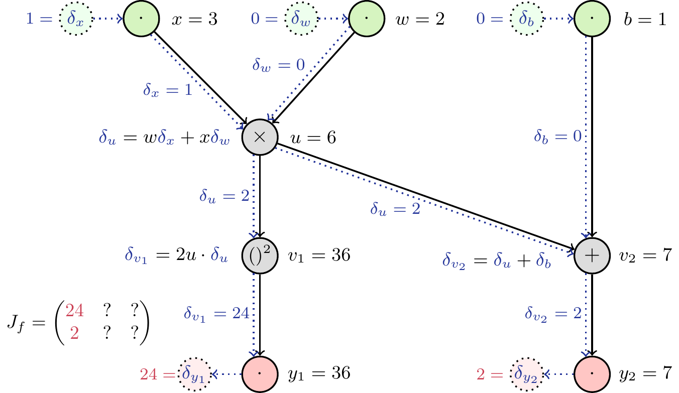
Code
\definecolor{mygreen}{HTML}{d6f4c0}
\definecolor{mypink}{HTML}{ffc6c4}
\definecolor{mygrey}{HTML}{dddddd}
\definecolor{mylightgreen}{HTML}{eeffee}
\definecolor{myred}{HTML}{ffeeee}
\definecolor{dcol}{HTML}{223399}
\definecolor{BrickRed}{rgb}{0.8, 0.25, 0.33}

\usetikzlibrary{positioning,graphdrawing,graphs,quotes}
\usegdlibrary{layered}
\tikzstyle{comp} = [draw, rectangle, rounded corners]

\tikzstyle{m} = [draw, circle, minimum size=0.6cm, inner xsep=0mm, inner ysep=0mm]
\tikzstyle{inp} = [m, fill=mygreen]
\tikzstyle{outp} = [m, fill=mypink]
\tikzstyle{op} = [m, fill=mygrey]
\tikzstyle{dl} = [draw, circle, dotted, fill=mylightgreen, minimum size=0.55cm, xshift=-0.1cm,font=\small,inner ysep=0, inner xsep=0, text=dcol]
\tikzstyle{dt} = [dl,xshift=0.1cm]
\tikzstyle{dr} = [dl, fill=myred]
\tikzstyle{eq} = [font=\small,align=center]
\tikzstyle{eqr} = [eq,xshift=-0.1cm]
\tikzstyle{eql} = [eq,xshift=0.1cm]
\tikzstyle{diff} = [->, dotted,swap,font=\footnotesize, inner xsep=0.5mm, inner ysep=0.1mm, text=dcol, dcol]
\tikzstyle{dval} = [font=\footnotesize,xshift=0.38cm,text=dcol]
\tikzstyle{dtval} = [font=\footnotesize,xshift=-0.35cm,text=dcol]

\newcounter{x}
\newcounter{w}
\newcounter{b}
\newcounter{u}
\newcounter{vone}
\newcounter{vtwo}

\newcounter{dx}
\newcounter{dw}
\newcounter{db}
\newcounter{du}
\newcounter{dvone}
\newcounter{dvtwo}
\newcounter{dyone}
\newcounter{dytwo}

\setcounter{x}{3}
\setcounter{w}{2}
\setcounter{b}{1}

\setcounter{dx}{0}
\setcounter{dw}{1}
\setcounter{db}{0}

\begin{tikzpicture}[thick]
        \setcounter{u}{\numexpr \thex * \thew \relax}
    \setcounter{vone}{\numexpr \theu * \theu \relax}
    \setcounter{vtwo}{\numexpr \theb + \theu \relax}

    \setcounter{du}{\numexpr \thew * \thedx + \thex * \thedw \relax}
    \setcounter{dvone}{\numexpr \thedu * 2 * \theu \relax}
    \setcounter{dvtwo}{\numexpr \thedu + \thedb \relax}
    \setcounter{dyone}{\thedvone}
    \setcounter{dytwo}{\thedvtwo}
    \graph[layered layout, grow=down, nodes={draw, circle}, sibling distance=3.8cm, level distance=2cm] {
        { [same layer] x[inp, as={$\cdot$}], w[inp, as={$\cdot$}], b[inp, as={$\cdot$}] };
        { [same layer] prod[op,as=$\times$, xshift=-1.8cm] };
        { [same layer] v2[op, as=$+$], v1[op, as=\small$()^2$, xshift=-1.8cm]};
        { [same layer] y1[outp, as={$\cdot$}, xshift=-1.8cm], y2[outp, as={$\cdot$}] };


        {b, prod} -> v2 -> y2;
        prod -> v1 -> y1;
        {x, w} -> prod;

    };
    % Input differentials
    \node [left of=x,dl](dx) {$\delta_x$};
    \node [left of=dx,dval](dxval) {$\thedx=$};
    \draw[diff] (dx) -- (x);
    \node [left of=w,dl](dw) {$\delta_w$};
    \node [left of=dw,dval](dwval) {$\thedw=$};
    \draw[diff] (dw) -- (w);
    \node [left of=b,dl](db) {$\delta_b$};
    \node [left of=db,dval](dbval) {$\thedb=$};
    \draw[diff] (db) -- (b);
    % Values of inputs
    \node [right of=x,eqr](xval) {$x=\thex$};
    \node [right of=w,eqr](wval) {$w=\thew$};
    \node [right of=b,eqr](bval) {$b=\theb$};
    % product
    \node [right of=prod,eqr](prodval) {$u=\theu$};
    \node [left of=prod,eql,align=center,xshift=-0.7cm](du) {$\color{dcol}\delta_u\color{black}=w\color{dcol}\delta_x\color{black}+x\color{dcol}\delta_w$};
    % v1
    \node [right of=v1,eqr,xshift=0.1cm](v1val) {$v_1=\thevone$};
    \node [left of=v1,eql,xshift=-0.5cm](dyone) {$\color{dcol}\delta_{v_1}\color{black}=2u\cdot\color{dcol}\delta_u$};
    % v2
    \node [right of=v2,eqr](v2val) {$v_2=\thevtwo$};
    \node [left of=v2,eql,xshift=-0.7cm,yshift=-0.1cm](dytwo) {$\color{dcol}\delta_{v_2}\color{black}=\color{dcol}\delta_u\color{black}+\color{dcol}\delta_b$};
    % Outputs
    \node [left of=y1,dr](dy1) {$\delta_{y_1}$};
    \node [right of=y1,eqr,xshift=0.1cm](y1val) {$y_1=\thevone$};
    \draw[diff] (y1) -- (dy1);
    \node [left of=dy1,dval](dy1val) {$\color{BrickRed}\thedvone=$};
    \node [left of=y2,dr](dy2) {$\delta_{y_2}$};
    \node [right of=y2,eqr](y2val) {$y_2=\thevtwo$};
    \draw[diff] (y2) -- (dy2);
    \node [left of=dy2,dval](dy2val) {$\color{BrickRed}\thedytwo=$};

    % Path of differentials
    \draw (x.300) edge[diff,"$\delta_x=\thedx$"] (prod.155);
    \draw (prod.250) edge[diff,"$\delta_u=\thedu$"] (v1.110);
    \draw (v1.250) edge[diff,"$\delta_{v_1}=\thedvone$"] (y1.110);
    \draw (w.205) edge[diff,"$\delta_w=\thedw$"] (prod.65);
    \draw (b.250) edge[diff,"$\delta_b=\thedb$"] (v2.110);
    \draw (v2.250) edge[diff,"$\delta_{v_2}=\thedytwo$"] (y2.110);
    \draw (prod.325) edge[diff,"$\delta_u=\thedu$"] (v2.175);

    \node[xshift=1.5cm,yshift=-2.6cm,scale=0.9] at (current page.south west){%
        $%
        J_f = %
        \begin{pmatrix}%
            \color{BrickRed}24 & \color{BrickRed}36 & ? \\%
            \color{BrickRed}2 & \color{BrickRed}3 & ?%
        \end{pmatrix}$};
\end{tikzpicture}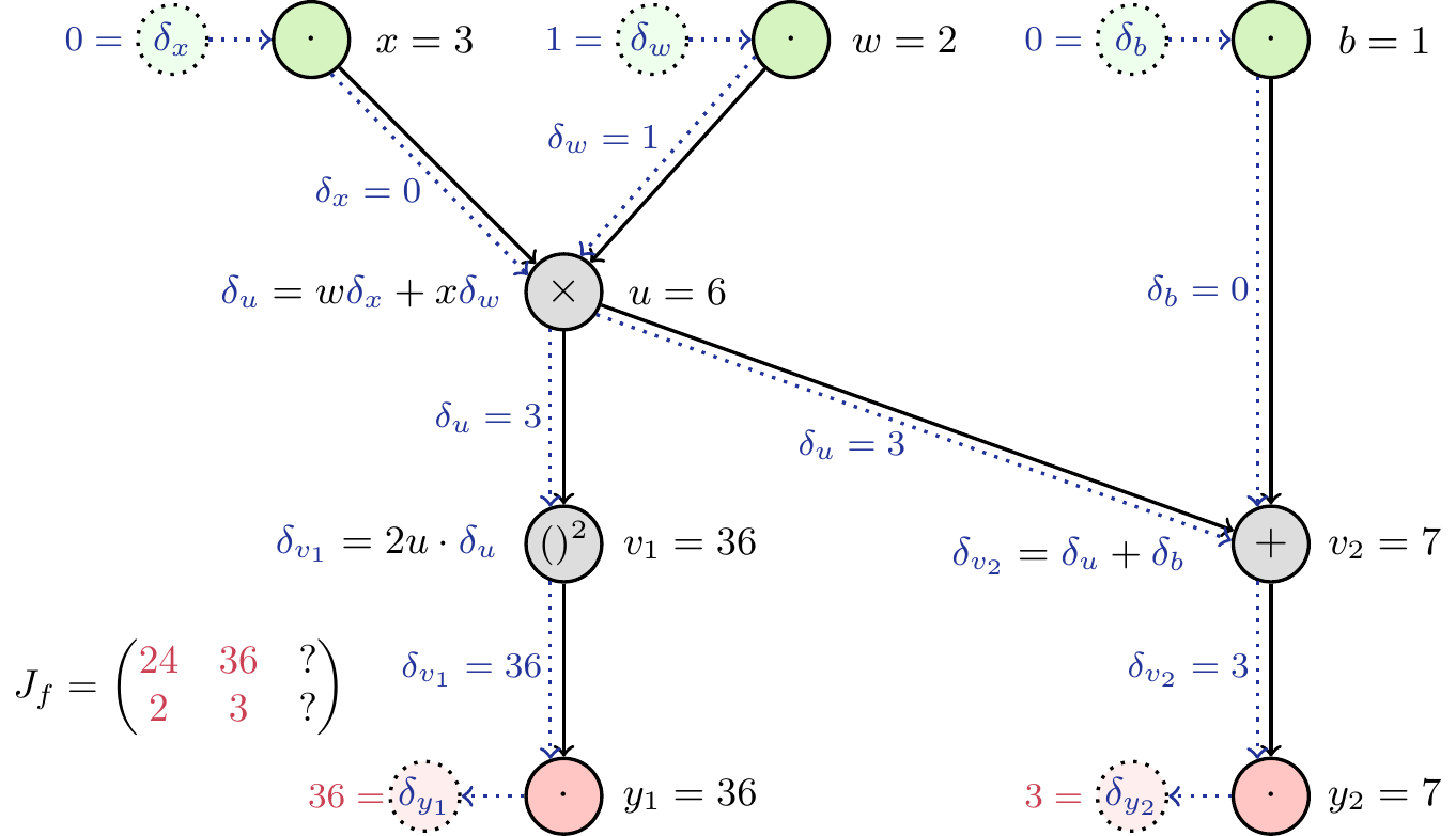
Code
\definecolor{mygreen}{HTML}{d6f4c0}
\definecolor{mypink}{HTML}{ffc6c4}
\definecolor{mygrey}{HTML}{dddddd}
\definecolor{mylightgreen}{HTML}{eeffee}
\definecolor{myred}{HTML}{ffeeee}
\definecolor{dcol}{HTML}{223399}
\definecolor{BrickRed}{rgb}{0.8, 0.25, 0.33}

\usetikzlibrary{positioning,graphdrawing,graphs,quotes}
\usegdlibrary{layered}
\tikzstyle{comp} = [draw, rectangle, rounded corners]

\tikzstyle{m} = [draw, circle, minimum size=0.6cm, inner xsep=0mm, inner ysep=0mm]
\tikzstyle{inp} = [m, fill=mygreen]
\tikzstyle{outp} = [m, fill=mypink]
\tikzstyle{op} = [m, fill=mygrey]
\tikzstyle{dl} = [draw, circle, dotted, fill=mylightgreen, minimum size=0.55cm, xshift=-0.1cm,font=\small,inner ysep=0, inner xsep=0, text=dcol]
\tikzstyle{dt} = [dl,xshift=0.1cm]
\tikzstyle{dr} = [dl, fill=myred]
\tikzstyle{eq} = [font=\small,align=center]
\tikzstyle{eqr} = [eq,xshift=-0.1cm]
\tikzstyle{eql} = [eq,xshift=0.1cm]
\tikzstyle{diff} = [->, dotted,swap,font=\footnotesize, inner xsep=0.5mm, inner ysep=0.1mm, text=dcol, dcol]
\tikzstyle{dval} = [font=\footnotesize,xshift=0.38cm,text=dcol]
\tikzstyle{dtval} = [font=\footnotesize,xshift=-0.35cm,text=dcol]

\newcounter{x}
\newcounter{w}
\newcounter{b}
\newcounter{u}
\newcounter{vone}
\newcounter{vtwo}

\newcounter{dx}
\newcounter{dw}
\newcounter{db}
\newcounter{du}
\newcounter{dvone}
\newcounter{dvtwo}
\newcounter{dyone}
\newcounter{dytwo}

\setcounter{x}{3}
\setcounter{w}{2}
\setcounter{b}{1}

\setcounter{dx}{0}
\setcounter{dw}{0}
\setcounter{db}{1}

\begin{tikzpicture}[thick]
        \setcounter{u}{\numexpr \thex * \thew \relax}
    \setcounter{vone}{\numexpr \theu * \theu \relax}
    \setcounter{vtwo}{\numexpr \theb + \theu \relax}

    \setcounter{du}{\numexpr \thew * \thedx + \thex * \thedw \relax}
    \setcounter{dvone}{\numexpr \thedu * 2 * \theu \relax}
    \setcounter{dvtwo}{\numexpr \thedu + \thedb \relax}
    \setcounter{dyone}{\thedvone}
    \setcounter{dytwo}{\thedvtwo}
    \graph[layered layout, grow=down, nodes={draw, circle}, sibling distance=3.8cm, level distance=2cm] {
        { [same layer] x[inp, as={$\cdot$}], w[inp, as={$\cdot$}], b[inp, as={$\cdot$}] };
        { [same layer] prod[op,as=$\times$, xshift=-1.8cm] };
        { [same layer] v2[op, as=$+$], v1[op, as=\small$()^2$, xshift=-1.8cm]};
        { [same layer] y1[outp, as={$\cdot$}, xshift=-1.8cm], y2[outp, as={$\cdot$}] };


        {b, prod} -> v2 -> y2;
        prod -> v1 -> y1;
        {x, w} -> prod;

    };
    % Input differentials
    \node [left of=x,dl](dx) {$\delta_x$};
    \node [left of=dx,dval](dxval) {$\thedx=$};
    \draw[diff] (dx) -- (x);
    \node [left of=w,dl](dw) {$\delta_w$};
    \node [left of=dw,dval](dwval) {$\thedw=$};
    \draw[diff] (dw) -- (w);
    \node [left of=b,dl](db) {$\delta_b$};
    \node [left of=db,dval](dbval) {$\thedb=$};
    \draw[diff] (db) -- (b);
    % Values of inputs
    \node [right of=x,eqr](xval) {$x=\thex$};
    \node [right of=w,eqr](wval) {$w=\thew$};
    \node [right of=b,eqr](bval) {$b=\theb$};
    % product
    \node [right of=prod,eqr](prodval) {$u=\theu$};
    \node [left of=prod,eql,align=center,xshift=-0.7cm](du) {$\color{dcol}\delta_u\color{black}=w\color{dcol}\delta_x\color{black}+x\color{dcol}\delta_w$};
    % v1
    \node [right of=v1,eqr,xshift=0.1cm](v1val) {$v_1=\thevone$};
    \node [left of=v1,eql,xshift=-0.5cm](dyone) {$\color{dcol}\delta_{v_1}\color{black}=2u\cdot\color{dcol}\delta_u$};
    % v2
    \node [right of=v2,eqr](v2val) {$v_2=\thevtwo$};
    \node [left of=v2,eql,xshift=-0.7cm,yshift=-0.1cm](dytwo) {$\color{dcol}\delta_{v_2}\color{black}=\color{dcol}\delta_u\color{black}+\color{dcol}\delta_b$};
    % Outputs
    \node [left of=y1,dr](dy1) {$\delta_{y_1}$};
    \node [right of=y1,eqr,xshift=0.1cm](y1val) {$y_1=\thevone$};
    \draw[diff] (y1) -- (dy1);
    \node [left of=dy1,dval](dy1val) {$\color{BrickRed}\thedvone=$};
    \node [left of=y2,dr](dy2) {$\delta_{y_2}$};
    \node [right of=y2,eqr](y2val) {$y_2=\thevtwo$};
    \draw[diff] (y2) -- (dy2);
    \node [left of=dy2,dval](dy2val) {$\color{BrickRed}\thedytwo=$};

    % Path of differentials
    \draw (x.300) edge[diff,"$\delta_x=\thedx$"] (prod.155);
    \draw (prod.250) edge[diff,"$\delta_u=\thedu$"] (v1.110);
    \draw (v1.250) edge[diff,"$\delta_{v_1}=\thedvone$"] (y1.110);
    \draw (w.205) edge[diff,"$\delta_w=\thedw$"] (prod.65);
    \draw (b.250) edge[diff,"$\delta_b=\thedb$"] (v2.110);
    \draw (v2.250) edge[diff,"$\delta_{v_2}=\thedytwo$"] (y2.110);
    \draw (prod.325) edge[diff,"$\delta_u=\thedu$"] (v2.175);

    \node[xshift=1.5cm,yshift=-2.6cm,scale=0.9] at (current page.south west){%
        $%
        J_f = %
        \begin{pmatrix}%
            \color{BrickRed}24 & \color{BrickRed}36 & \color{BrickRed}0 \\%
            \color{BrickRed}2 & \color{BrickRed}3 & \color{BrickRed}1%
        \end{pmatrix}$};
\end{tikzpicture}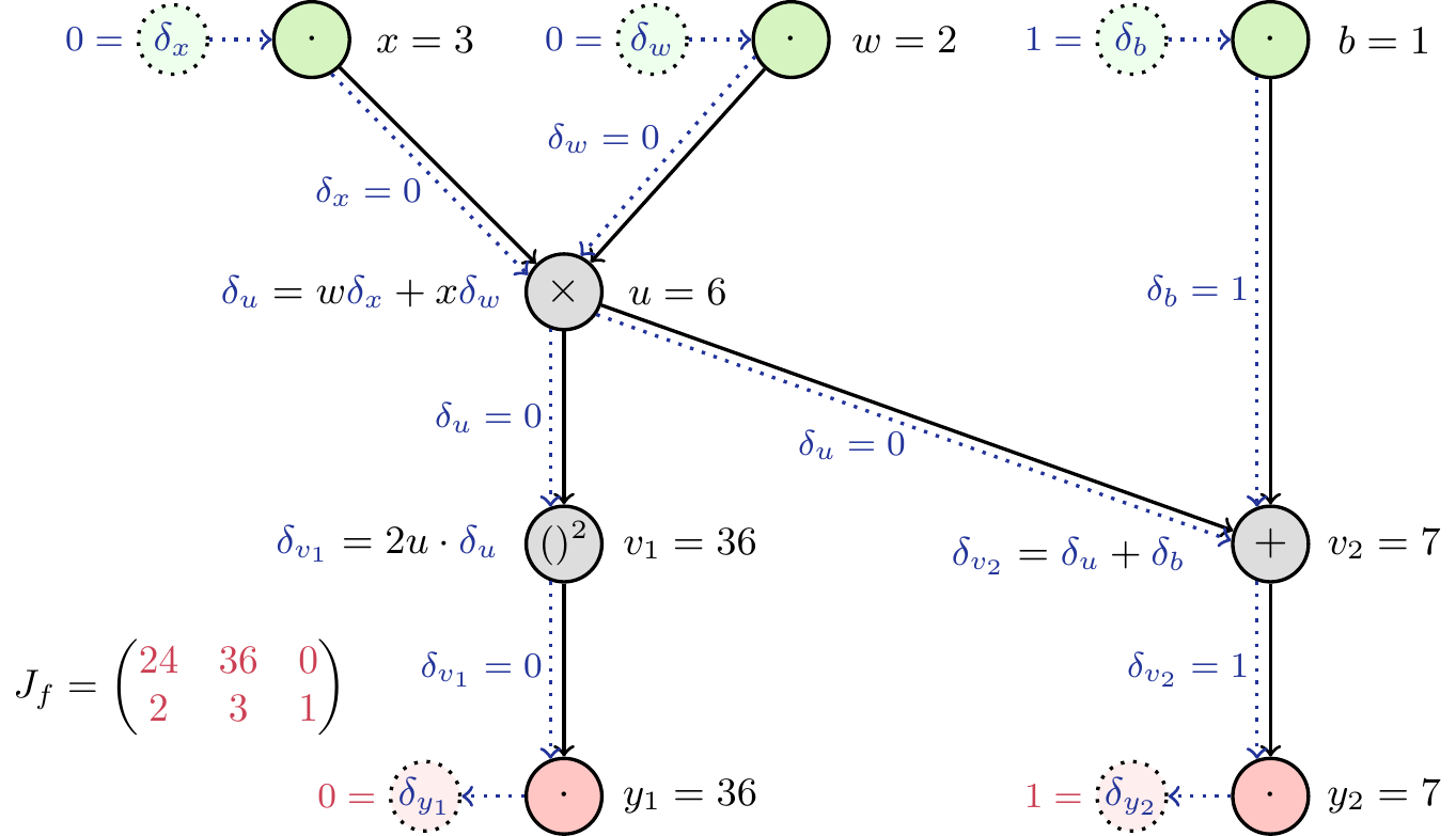
Reverse mode
In a similar fashion, we can use Equation 3 to construct the graph for the reverse mode (Figure 11). Computing the partial derivatives is again straight-forward (Figure 12). As shown above, by initializing the differentials to one at the output, we can read off the derivative at the input. Again, the case that multiple outputs are present will lead to interference during the backward pass, so we only set one at a time to one, which allows us to obtain one row of the Jacobian. Therefore we need number of outputs (here: two) backward passes to obtain the full Jacobian. In addition we have to do one forward pass to obtain the intermediate values which are needed to calculate the partial derivatives.
Code
\definecolor{mygreen}{HTML}{d6f4c0}
\definecolor{mypink}{HTML}{ffc6c4}
\definecolor{mygrey}{HTML}{dddddd}
\definecolor{mylightgreen}{HTML}{eeffee}
\definecolor{myred}{HTML}{ffeeee}
\definecolor{dcol}{HTML}{223399}

\usetikzlibrary{positioning,graphdrawing,graphs,quotes}
\usegdlibrary{layered}
\tikzstyle{comp} = [draw, rectangle, rounded corners]

\tikzstyle{m} = [draw, circle, minimum size=0.6cm, inner xsep=0mm, inner ysep=0mm]
\tikzstyle{inp} = [m, fill=mygreen]
\tikzstyle{outp} = [m, fill=mypink]
\tikzstyle{op} = [m, fill=mygrey]
\tikzstyle{dl} = [draw, circle, dotted, fill=mylightgreen, minimum size=0.55cm, xshift=-0.1cm,font=\small,inner ysep=0, inner xsep=0, text=dcol]
\tikzstyle{dt} = [dl,xshift=0.1cm]
\tikzstyle{dr} = [dl, fill=myred]
\tikzstyle{eq} = [font=\small,align=center]
\tikzstyle{eqr} = [eq,xshift=-0.1cm]
\tikzstyle{eql} = [eq,xshift=0.1cm]
\tikzstyle{diff} = [<-, dotted,swap,font=\footnotesize, inner xsep=0.5mm, inner ysep=0.1mm, text=dcol, dcol]
\tikzstyle{dval} = [font=\footnotesize,xshift=0.38cm,text=dcol]
\tikzstyle{dtval} = [font=\footnotesize,xshift=-0.35cm,text=dcol]

\newcounter{x}
\newcounter{w}
\newcounter{b}
\newcounter{u}
\newcounter{vone}
\newcounter{vtwo}

\newcounter{dx}
\newcounter{dw}
\newcounter{db}
\newcounter{du}
\newcounter{dvone}
\newcounter{dvtwo}
\newcounter{dyone}
\newcounter{dytwo}

\setcounter{x}{3}
\setcounter{w}{2}
\setcounter{b}{1}

\begin{tikzpicture}[thick]
    \setcounter{u}{\numexpr \thex * \thew \relax}
    \setcounter{vone}{\numexpr \theu * \theu \relax}
    \setcounter{vtwo}{\numexpr \theb + \theu \relax}


    \setcounter{dvone}{\thedyone}
    \setcounter{dvtwo}{\thedytwo}

    \setcounter{du}{\numexpr \thedyone * 2 * \theu + \thedytwo \relax}
    \setcounter{dx}{\numexpr \thedu * \thew \relax}
    \setcounter{dw}{\numexpr \thedu * \thex \relax}
    \setcounter{db}{\thedvtwo}
    \setcounter{dvtwo}{\thedytwo}
    \graph[layered layout, grow=down, nodes={draw, circle}, sibling distance=3.8cm, level distance=2cm] {
        { [same layer] x[inp, as={$\cdot$}], w[inp, as={$\cdot$}], b[inp, as={$\cdot$}] };
        { [same layer] prod[op,as=$\times$, xshift=-1.8cm] };
        { [same layer] v2[op, as=$+$], v1[op, as=\small$()^2$, xshift=-1.8cm]};
        { [same layer] y1[outp, as={$\cdot$}, xshift=-1.8cm], y2[outp, as={$\cdot$}] };


        {b, prod} -> v2 -> y2;
        prod -> v1 -> y1;
        {x, w} -> prod;

    };
    % Input differentials
    \node [left of=x,eql,xshift=-0.3cm](dxcalc) {$\color{dcol}\bar\delta_{x}\color{black}=\color{dcol}\bar\delta_{u}\color{black}\frac{\partial u}{\partial x}$};
    \node [left of=w,eql,xshift=-0.45cm](dxcalc) {$\color{dcol}\bar\delta_{w}\color{black}=\color{dcol}\bar\delta_{u}\color{black}\cdot \frac{\partial u}{\partial w}$};
    \node [left of=b,eql,xshift=-0.3cm](dxcalc) {$\color{dcol}\bar\delta_{b}\color{black}=\color{dcol}\bar\delta_{v_2}\color{black}\frac{\partial v_2}{\partial b}$};
    % Values of inputs
    \node [right of=x,eqr](xval) {$x=\thex$};
    \node [right of=w,eqr](wval) {$w=\thew$};
    \node [right of=b,eqr](bval) {$b=\theb$};
    % product
    \node [right of=prod,eqr](prodval) {$u=xw$};
    \node [right of=prod,eql,align=center,xshift=-3.1cm](du) {$\color{dcol}\bar\delta_u\color{black}=\color{dcol}\bar\delta_{v_1}\color{black}\frac{\partial v_1}{\partial u}+\color{dcol}\bar\delta_{v_2}\color{black}\frac{\partial v_2}{\partial u}$};
    % v1
    \node [right of=v1,eqr,xshift=0.1cm](v1val) {$v_1=u^2$};
    \node [left of=v1,eql,xshift=-0.4cm](dyone) {$\color{dcol}\bar\delta_{v_1}\color{black}=\color{dcol}\bar\delta_{y_1}\color{black}\frac{\partial y_1}{\partial v_1}$};
    % v2
    \node [right of=v2,eqr,xshift=0.3cm](v2val) {$v_2=u+b$};
    \node [left of=v2,eql,xshift=-0.5cm,yshift=-0.1cm](dytwo) {$\color{dcol}\bar\delta_{v_2}\color{black}=\color{dcol}\bar\delta_{y_2}\color{black}\frac{\partial y_2}{\partial v_2}$};
    % Outputs
    \node [left of=y1,dr](dy1) {$\bar\delta_{y_1}$};
    \node [right of=y1,eqr,xshift=0.1cm](y1val) {$y_1=v_1$};
    \draw[diff] (y1) -- (dy1);
    \node [left of=dy1,dval](dy1val) {};
    \node [left of=y2,dr](dy2) {$\bar\delta_{y_2}$};
    \node [right of=y2,eqr](y2val) {$y_2=v_2$};
    \draw[diff] (y2) -- (dy2);
    \node [left of=dy2,dval](dy2val) {};

    % Path of differentials
    \draw (x.300) edge[diff,"$\bar\delta_u$"] (prod.155);
    \draw (prod.250) edge[diff,"$\bar\delta_{v_1}$"] (v1.110);
    \draw (v1.250) edge[diff,"$\bar\delta_{y_1}$"] (y1.110);
    \draw (w.205) edge[diff,"$\bar\delta_u$"] (prod.65);
    \draw (b.250) edge[diff,"$\bar\delta_{v_2}$"] (v2.110);
    \draw (v2.250) edge[diff,"$\bar\delta_{y_2}$"] (y2.110);
    \draw (prod.325) edge[diff,"$\bar\delta_{v_2}$"] (v2.175);


    \node[xshift=1.5cm,yshift=-2.6cm,scale=0.9] at (current page.south west){%
        $%
        J_f = %
        \begin{pmatrix}%
            ? & ? & ? \\%
            ? & ? & ?%
        \end{pmatrix}$};
\end{tikzpicture}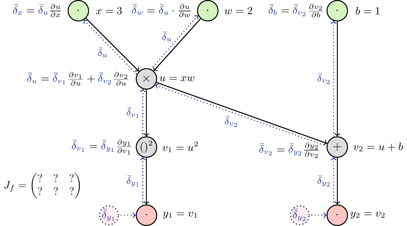
Code
\definecolor{mygreen}{HTML}{d6f4c0}
\definecolor{mypink}{HTML}{ffc6c4}
\definecolor{mygrey}{HTML}{dddddd}
\definecolor{mylightgreen}{HTML}{eeffee}
\definecolor{myred}{HTML}{ffeeee}
\definecolor{dcol}{HTML}{223399}

\usetikzlibrary{positioning,graphdrawing,graphs,quotes}
\usegdlibrary{layered}
\tikzstyle{comp} = [draw, rectangle, rounded corners]

\tikzstyle{m} = [draw, circle, minimum size=0.6cm, inner xsep=0mm, inner ysep=0mm]
\tikzstyle{inp} = [m, fill=mygreen]
\tikzstyle{outp} = [m, fill=mypink]
\tikzstyle{op} = [m, fill=mygrey]
\tikzstyle{dl} = [draw, circle, dotted, fill=mylightgreen, minimum size=0.55cm, xshift=-0.1cm,font=\small,inner ysep=0, inner xsep=0, text=dcol]
\tikzstyle{dt} = [dl,xshift=0.1cm]
\tikzstyle{dr} = [dl, fill=myred]
\tikzstyle{eq} = [font=\small,align=center]
\tikzstyle{eqr} = [eq,xshift=-0.1cm]
\tikzstyle{eql} = [eq,xshift=0.1cm]
\tikzstyle{diff} = [<-, dotted,swap,font=\footnotesize, inner xsep=0.5mm, inner ysep=0.1mm, text=dcol, dcol]
\tikzstyle{dval} = [font=\footnotesize,xshift=0.38cm,text=dcol]
\tikzstyle{dtval} = [font=\footnotesize,xshift=-0.35cm,text=dcol]

\newcounter{x}
\newcounter{w}
\newcounter{b}
\newcounter{u}
\newcounter{vone}
\newcounter{vtwo}

\newcounter{dx}
\newcounter{dw}
\newcounter{db}
\newcounter{du}
\newcounter{dvone}
\newcounter{dvtwo}
\newcounter{dyone}
\newcounter{dytwo}

\setcounter{x}{3}
\setcounter{w}{2}
\setcounter{b}{1}

\begin{tikzpicture}[thick]
    \setcounter{u}{\numexpr \thex * \thew \relax}
    \setcounter{vone}{\numexpr \theu * \theu \relax}
    \setcounter{vtwo}{\numexpr \theb + \theu \relax}


    \setcounter{dvone}{\thedyone}
    \setcounter{dvtwo}{\thedytwo}

    \setcounter{du}{\numexpr \thedyone * 2 * \theu + \thedytwo \relax}
    \setcounter{dx}{\numexpr \thedu * \thew \relax}
    \setcounter{dw}{\numexpr \thedu * \thex \relax}
    \setcounter{db}{\thedvtwo}
    \setcounter{dvtwo}{\thedytwo}
    \graph[layered layout, grow=down, nodes={draw, circle}, sibling distance=3.8cm, level distance=2cm] {
        { [same layer] x[inp, as={$\cdot$}], w[inp, as={$\cdot$}], b[inp, as={$\cdot$}] };
        { [same layer] prod[op,as=$\times$, xshift=-1.8cm] };
        { [same layer] v2[op, as=$+$], v1[op, as=\small$()^2$, xshift=-1.8cm]};
        { [same layer] y1[outp, as={$\cdot$}, xshift=-1.8cm], y2[outp, as={$\cdot$}] };


        {b, prod} -> v2 -> y2;
        prod -> v1 -> y1;
        {x, w} -> prod;

    };
    % Input differentials
    \node [left of=x,eql,xshift=-0.3cm](dxcalc) {$\color{dcol}\bar\delta_{x}\color{black}=\color{dcol}\bar\delta_{u}\color{black}\cdot w$};
    \node [left of=w,eql,xshift=-0.3cm](dxcalc) {$\color{dcol}\bar\delta_{w}\color{black}=\color{dcol}\bar\delta_{u}\color{black}\cdot x$};
    \node [left of=b,eql,xshift=-0.1cm](dxcalc) {$\color{dcol}\bar\delta_{b}\color{black}=\color{dcol}\bar\delta_{v_2}$};
    % Values of inputs
    \node [right of=x,eqr](xval) {$x=\thex$};
    \node [right of=w,eqr](wval) {$w=\thew$};
    \node [right of=b,eqr](bval) {$b=\theb$};
    % product
    \node [right of=prod,eqr](prodval) {$u=xw$};
    \node [right of=prod,eql,align=center,xshift=-2.9cm](du) {$\color{dcol}\bar\delta_u\color{black}=\color{dcol}\bar\delta_{v_1}\color{black}\cdot2u+\color{dcol}\bar\delta_{v_2}$};
    % v1
    \node [right of=v1,eqr,xshift=0.1cm](v1val) {$v_1=u^2$};
    \node [left of=v1,eql,xshift=-0.1cm](dyone) {$\color{dcol}\bar\delta_{v_1}\color{black}=\color{dcol}\bar\delta_{y_1}$};
    % v2
    \node [right of=v2,eqr,xshift=0.3cm](v2val) {$v_2=u+b$};
    \node [left of=v2,eql,xshift=-0.2cm,yshift=-0.1cm](dytwo) {$\color{dcol}\bar\delta_{v_2}\color{black}=\color{dcol}\bar\delta_{y_2}$};
    % Outputs
    \node [left of=y1,dr](dy1) {$\bar\delta_{y_1}$};
    \node [right of=y1,eqr,xshift=0.1cm](y1val) {$y_1=v_1$};
    \draw[diff] (y1) -- (dy1);
    \node [left of=dy1,dval](dy1val) {};
    \node [left of=y2,dr](dy2) {$\bar\delta_{y_2}$};
    \node [right of=y2,eqr](y2val) {$y_2=v_2$};
    \draw[diff] (y2) -- (dy2);
    \node [left of=dy2,dval](dy2val) {};

    % Path of differentials
    \draw (x.300) edge[diff,"$\bar\delta_u$"] (prod.155);
    \draw (prod.250) edge[diff,"$\bar\delta_{v_1}$"] (v1.110);
    \draw (v1.250) edge[diff,"$\bar\delta_{y_1}$"] (y1.110);
    \draw (w.205) edge[diff,"$\bar\delta_u$"] (prod.65);
    \draw (b.250) edge[diff,"$\bar\delta_{v_2}$"] (v2.110);
    \draw (v2.250) edge[diff,"$\bar\delta_{y_2}$"] (y2.110);
    \draw (prod.325) edge[diff,"$\bar\delta_{v_2}$"] (v2.175);

    \node[xshift=1.5cm,yshift=-2.6cm,scale=0.9] at (current page.south west){%
        $%
        J_f = %
        \begin{pmatrix}%
            ? & ? & ? \\%
            ? & ? & ?%
        \end{pmatrix}$};
\end{tikzpicture}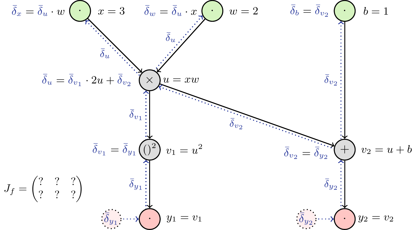
Code
\definecolor{mygreen}{HTML}{d6f4c0}
\definecolor{mypink}{HTML}{ffc6c4}
\definecolor{mygrey}{HTML}{dddddd}
\definecolor{mylightgreen}{HTML}{eeffee}
\definecolor{myred}{HTML}{ffeeee}
\definecolor{dcol}{HTML}{223399}
\definecolor{BrickRed}{rgb}{0.8, 0.25, 0.33}
\definecolor{OliveGreen}{rgb}{0.0, 0.4, 0.0}

\usetikzlibrary{positioning,graphdrawing,graphs,quotes}
\usegdlibrary{layered}
\tikzstyle{comp} = [draw, rectangle, rounded corners]

\tikzstyle{m} = [draw, circle, minimum size=0.6cm, inner xsep=0mm, inner ysep=0mm]
\tikzstyle{inp} = [m, fill=mygreen]
\tikzstyle{outp} = [m, fill=mypink]
\tikzstyle{op} = [m, fill=mygrey]
\tikzstyle{dl} = [draw, circle, dotted, fill=mylightgreen, minimum size=0.55cm, xshift=-0.1cm,font=\small,inner ysep=0, inner xsep=0, text=dcol]
\tikzstyle{dt} = [dl,xshift=0.1cm]
\tikzstyle{dr} = [dl, fill=myred]
\tikzstyle{eq} = [font=\small,align=center]
\tikzstyle{eqr} = [eq,xshift=-0.1cm]
\tikzstyle{eql} = [eq,xshift=0.1cm]
\tikzstyle{diff} = [<-, dotted,swap,font=\footnotesize, inner xsep=0.5mm, inner ysep=0.1mm, text=dcol, dcol]
\tikzstyle{dval} = [font=\footnotesize,xshift=0.38cm,text=dcol]
\tikzstyle{dtval} = [font=\footnotesize,xshift=-0.35cm,text=dcol]

\newcounter{x}
\newcounter{w}
\newcounter{b}
\newcounter{u}
\newcounter{vone}
\newcounter{vtwo}

\newcounter{dx}
\newcounter{dw}
\newcounter{db}
\newcounter{du}
\newcounter{dvone}
\newcounter{dvtwo}
\newcounter{dyone}
\newcounter{dytwo}

\setcounter{x}{3}
\setcounter{w}{2}
\setcounter{b}{1}

\setcounter{dyone}{1}
\setcounter{dytwo}{0}

\begin{tikzpicture}[thick]
    \setcounter{u}{\numexpr \thex * \thew \relax}
    \setcounter{vone}{\numexpr \theu * \theu \relax}
    \setcounter{vtwo}{\numexpr \theb + \theu \relax}


    \setcounter{dvone}{\thedyone}
    \setcounter{dvtwo}{\thedytwo}

    \setcounter{du}{\numexpr \thedyone * 2 * \theu + \thedytwo \relax}
    \setcounter{dx}{\numexpr \thedu * \thew \relax}
    \setcounter{dw}{\numexpr \thedu * \thex \relax}
    \setcounter{db}{\thedvtwo}
    \setcounter{dvtwo}{\thedytwo}
    \graph[layered layout, grow=down, nodes={draw, circle}, sibling distance=3.8cm, level distance=2cm] {
        { [same layer] x[inp, as={$\cdot$}], w[inp, as={$\cdot$}], b[inp, as={$\cdot$}] };
        { [same layer] prod[op,as=$\times$, xshift=-1.8cm] };
        { [same layer] v2[op, as=$+$], v1[op, as=\small$()^2$, xshift=-1.8cm]};
        { [same layer] y1[outp, as={$\cdot$}, xshift=-1.8cm], y2[outp, as={$\cdot$}] };


        {b, prod} -> v2 -> y2;
        prod -> v1 -> y1;
        {x, w} -> prod;

    };
    % Input differentials
    \node [above of=x,dt](dx) {$\bar\delta_x$};
    \node [right of=dx,dtval](dxval) {$=\color{OliveGreen}\thedx$};
    \node [left of=x,eql,xshift=-0.3cm](dxcalc) {$\color{dcol}\bar\delta_{x}\color{black}=\color{dcol}\bar\delta_{u}\color{black}\cdot w$};
    \draw[diff] (dx) -- (x);
    \node [above of=w,dt](dw) {$\bar\delta_w$};
    \node [right of=dw,dtval](dwval) {$=\color{OliveGreen}\thedw$};
    \node [left of=w,eql,xshift=-0.3cm](dxcalc) {$\color{dcol}\bar\delta_{w}\color{black}=\color{dcol}\bar\delta_{u}\color{black}\cdot x$};
    \draw[diff] (dw) -- (w);
    \node [above of=b,dt](db) {$\bar\delta_b$};
    \node [right of=db,dtval](dbval) {$=\color{OliveGreen}\thedb$};
    \node [left of=b,eql,xshift=-0.1cm](dxcalc) {$\color{dcol}\bar\delta_{b}\color{black}=\color{dcol}\bar\delta_{v_2}$};
    \draw[diff] (db) -- (b);
    % Values of inputs
    \node [right of=x,eqr](xval) {$x=\thex$};
    \node [right of=w,eqr](wval) {$w=\thew$};
    \node [right of=b,eqr](bval) {$b=\theb$};
    % product
    \node [right of=prod,eqr](prodval) {$u=\theu$};
    \node [right of=prod,eql,align=center,xshift=-2.9cm](du) {$\color{dcol}\bar\delta_u\color{black}=\color{dcol}\bar\delta_{v_1}\color{black}\cdot2u+\color{dcol}\bar\delta_{v_2}$};
    % v1
    \node [right of=v1,eqr,xshift=0.1cm](v1val) {$v_1=\thevone$};
    \node [left of=v1,eql,xshift=-0.1cm](dyone) {$\color{dcol}\bar\delta_{v_1}\color{black}=\color{dcol}\bar\delta_{y_1}$};
    % v2
    \node [right of=v2,eqr](v2val) {$v_2=\thevtwo$};
    \node [left of=v2,eql,xshift=-0.2cm,yshift=-0.1cm](dytwo) {$\color{dcol}\bar\delta_{v_2}\color{black}=\color{dcol}\bar\delta_{y_2}$};
    % Outputs
    \node [left of=y1,dr](dy1) {$\bar\delta_{y_1}$};
    \node [right of=y1,eqr,xshift=0.1cm](y1val) {$y_1=\thevone$};
    \draw[diff] (y1) -- (dy1);
    \node [left of=dy1,dval](dy1val) {$\thedvone=$};
    \node [left of=y2,dr](dy2) {$\bar\delta_{y_2}$};
    \node [right of=y2,eqr](y2val) {$y_2=\thevtwo$};
    \draw[diff] (y2) -- (dy2);
    \node [left of=dy2,dval](dy2val) {$\thedytwo=$};

    % Path of differentials
    \draw (x.300) edge[diff,"$\bar\delta_u=\thedu$"] (prod.155);
    \draw (prod.250) edge[diff,"$\bar\delta_{v_1}=\thedvone$"] (v1.110);
    \draw (v1.250) edge[diff,"$\bar\delta_{y_1}=\thedyone$"] (y1.110);
    \draw (w.205) edge[diff,"$\bar\delta_u=\thedu$"] (prod.65);
    \draw (b.250) edge[diff,"$\bar\delta_{v_2}=\thedvtwo$"] (v2.110);
    \draw (v2.250) edge[diff,"$\bar\delta_{y_2}=\thedytwo$"] (y2.110);
    \draw (prod.325) edge[diff,"$\bar\delta_{v_2}=\thedvtwo$"] (v2.175);

    \node[xshift=1.5cm,yshift=-2.6cm,scale=0.9] at (current page.south west){%
        $%
        J_f = %
        \begin{pmatrix}%
            \color{OliveGreen}24 & \color{OliveGreen}36 & \color{OliveGreen}0 \\%
            ?  & ? & ?%
        \end{pmatrix}$};
\end{tikzpicture}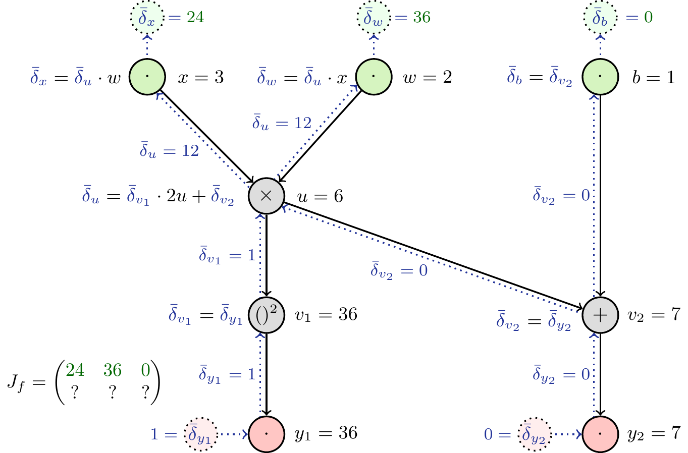
Code
\definecolor{mygreen}{HTML}{d6f4c0}
\definecolor{mypink}{HTML}{ffc6c4}
\definecolor{mygrey}{HTML}{dddddd}
\definecolor{mylightgreen}{HTML}{eeffee}
\definecolor{myred}{HTML}{ffeeee}
\definecolor{dcol}{HTML}{223399}
\definecolor{BrickRed}{rgb}{0.8, 0.25, 0.33}
\definecolor{OliveGreen}{rgb}{0.0, 0.4, 0.0}

\usetikzlibrary{positioning,graphdrawing,graphs,quotes}
\usegdlibrary{layered}
\tikzstyle{comp} = [draw, rectangle, rounded corners]

\tikzstyle{m} = [draw, circle, minimum size=0.6cm, inner xsep=0mm, inner ysep=0mm]
\tikzstyle{inp} = [m, fill=mygreen]
\tikzstyle{outp} = [m, fill=mypink]
\tikzstyle{op} = [m, fill=mygrey]
\tikzstyle{dl} = [draw, circle, dotted, fill=mylightgreen, minimum size=0.55cm, xshift=-0.1cm,font=\small,inner ysep=0, inner xsep=0, text=dcol]
\tikzstyle{dt} = [dl,xshift=0.1cm]
\tikzstyle{dr} = [dl, fill=myred]
\tikzstyle{eq} = [font=\small,align=center]
\tikzstyle{eqr} = [eq,xshift=-0.1cm]
\tikzstyle{eql} = [eq,xshift=0.1cm]
\tikzstyle{diff} = [<-, dotted,swap,font=\footnotesize, inner xsep=0.5mm, inner ysep=0.1mm, text=dcol, dcol]
\tikzstyle{dval} = [font=\footnotesize,xshift=0.38cm,text=dcol]
\tikzstyle{dtval} = [font=\footnotesize,xshift=-0.35cm,text=dcol]

\newcounter{x}
\newcounter{w}
\newcounter{b}
\newcounter{u}
\newcounter{vone}
\newcounter{vtwo}

\newcounter{dx}
\newcounter{dw}
\newcounter{db}
\newcounter{du}
\newcounter{dvone}
\newcounter{dvtwo}
\newcounter{dyone}
\newcounter{dytwo}

\setcounter{x}{3}
\setcounter{w}{2}
\setcounter{b}{1}

\setcounter{dyone}{0}
\setcounter{dytwo}{1}

\begin{tikzpicture}[thick]
    \setcounter{u}{\numexpr \thex * \thew \relax}
    \setcounter{vone}{\numexpr \theu * \theu \relax}
    \setcounter{vtwo}{\numexpr \theb + \theu \relax}


    \setcounter{dvone}{\thedyone}
    \setcounter{dvtwo}{\thedytwo}

    \setcounter{du}{\numexpr \thedyone * 2 * \theu + \thedytwo \relax}
    \setcounter{dx}{\numexpr \thedu * \thew \relax}
    \setcounter{dw}{\numexpr \thedu * \thex \relax}
    \setcounter{db}{\thedvtwo}
    \setcounter{dvtwo}{\thedytwo}
    \graph[layered layout, grow=down, nodes={draw, circle}, sibling distance=3.8cm, level distance=2cm] {
        { [same layer] x[inp, as={$\cdot$}], w[inp, as={$\cdot$}], b[inp, as={$\cdot$}] };
        { [same layer] prod[op,as=$\times$, xshift=-1.8cm] };
        { [same layer] v2[op, as=$+$], v1[op, as=\small$()^2$, xshift=-1.8cm]};
        { [same layer] y1[outp, as={$\cdot$}, xshift=-1.8cm], y2[outp, as={$\cdot$}] };


        {b, prod} -> v2 -> y2;
        prod -> v1 -> y1;
        {x, w} -> prod;

    };
    % Input differentials
    \node [above of=x,dt](dx) {$\bar\delta_x$};
    \node [right of=dx,dtval](dxval) {$=\color{OliveGreen}\thedx$};
    \node [left of=x,eql,xshift=-0.3cm](dxcalc) {$\color{dcol}\bar\delta_{x}\color{black}=\color{dcol}\bar\delta_{u}\color{black}\cdot w$};
    \draw[diff] (dx) -- (x);
    \node [above of=w,dt](dw) {$\bar\delta_w$};
    \node [right of=dw,dtval](dwval) {$=\color{OliveGreen}\thedw$};
    \node [left of=w,eql,xshift=-0.3cm](dxcalc) {$\color{dcol}\bar\delta_{w}\color{black}=\color{dcol}\bar\delta_{u}\color{black}\cdot x$};
    \draw[diff] (dw) -- (w);
    \node [above of=b,dt](db) {$\bar\delta_b$};
    \node [right of=db,dtval](dbval) {$=\color{OliveGreen}\thedb$};
    \node [left of=b,eql,xshift=-0.1cm](dxcalc) {$\color{dcol}\bar\delta_{b}\color{black}=\color{dcol}\bar\delta_{v_2}$};
    \draw[diff] (db) -- (b);
    % Values of inputs
    \node [right of=x,eqr](xval) {$x=\thex$};
    \node [right of=w,eqr](wval) {$w=\thew$};
    \node [right of=b,eqr](bval) {$b=\theb$};
    % product
    \node [right of=prod,eqr](prodval) {$u=\theu$};
    \node [right of=prod,eql,align=center,xshift=-2.9cm](du) {$\color{dcol}\bar\delta_u\color{black}=\color{dcol}\bar\delta_{v_1}\color{black}\cdot2u+\color{dcol}\bar\delta_{v_2}$};
    % v1
    \node [right of=v1,eqr,xshift=0.1cm](v1val) {$v_1=\thevone$};
    \node [left of=v1,eql,xshift=-0.1cm](dyone) {$\color{dcol}\bar\delta_{v_1}\color{black}=\color{dcol}\bar\delta_{y_1}$};
    % v2
    \node [right of=v2,eqr](v2val) {$v_2=\thevtwo$};
    \node [left of=v2,eql,xshift=-0.2cm,yshift=-0.1cm](dytwo) {$\color{dcol}\bar\delta_{v_2}\color{black}=\color{dcol}\bar\delta_{y_2}$};
    % Outputs
    \node [left of=y1,dr](dy1) {$\bar\delta_{y_1}$};
    \node [right of=y1,eqr,xshift=0.1cm](y1val) {$y_1=\thevone$};
    \draw[diff] (y1) -- (dy1);
    \node [left of=dy1,dval](dy1val) {$\thedvone=$};
    \node [left of=y2,dr](dy2) {$\bar\delta_{y_2}$};
    \node [right of=y2,eqr](y2val) {$y_2=\thevtwo$};
    \draw[diff] (y2) -- (dy2);
    \node [left of=dy2,dval](dy2val) {$\thedytwo=$};

    % Path of differentials
    \draw (x.300) edge[diff,"$\bar\delta_u=\thedu$"] (prod.155);
    \draw (prod.250) edge[diff,"$\bar\delta_{v_1}=\thedvone$"] (v1.110);
    \draw (v1.250) edge[diff,"$\bar\delta_{y_1}=\thedyone$"] (y1.110);
    \draw (w.205) edge[diff,"$\bar\delta_u=\thedu$"] (prod.65);
    \draw (b.250) edge[diff,"$\bar\delta_{v_2}=\thedvtwo$"] (v2.110);
    \draw (v2.250) edge[diff,"$\bar\delta_{y_2}=\thedytwo$"] (y2.110);
    \draw (prod.325) edge[diff,"$\bar\delta_{v_2}=\thedvtwo$"] (v2.175);

    \node[xshift=1.5cm,yshift=-2.6cm,scale=0.9] at (current page.south west){%
        $%
        J_f = %
        \begin{pmatrix}%
            \color{OliveGreen}24 & \color{OliveGreen}36 & \color{OliveGreen}0 \\%
            \color{OliveGreen}2 & \color{OliveGreen}3 & \color{OliveGreen}1%
        \end{pmatrix}$};
\end{tikzpicture}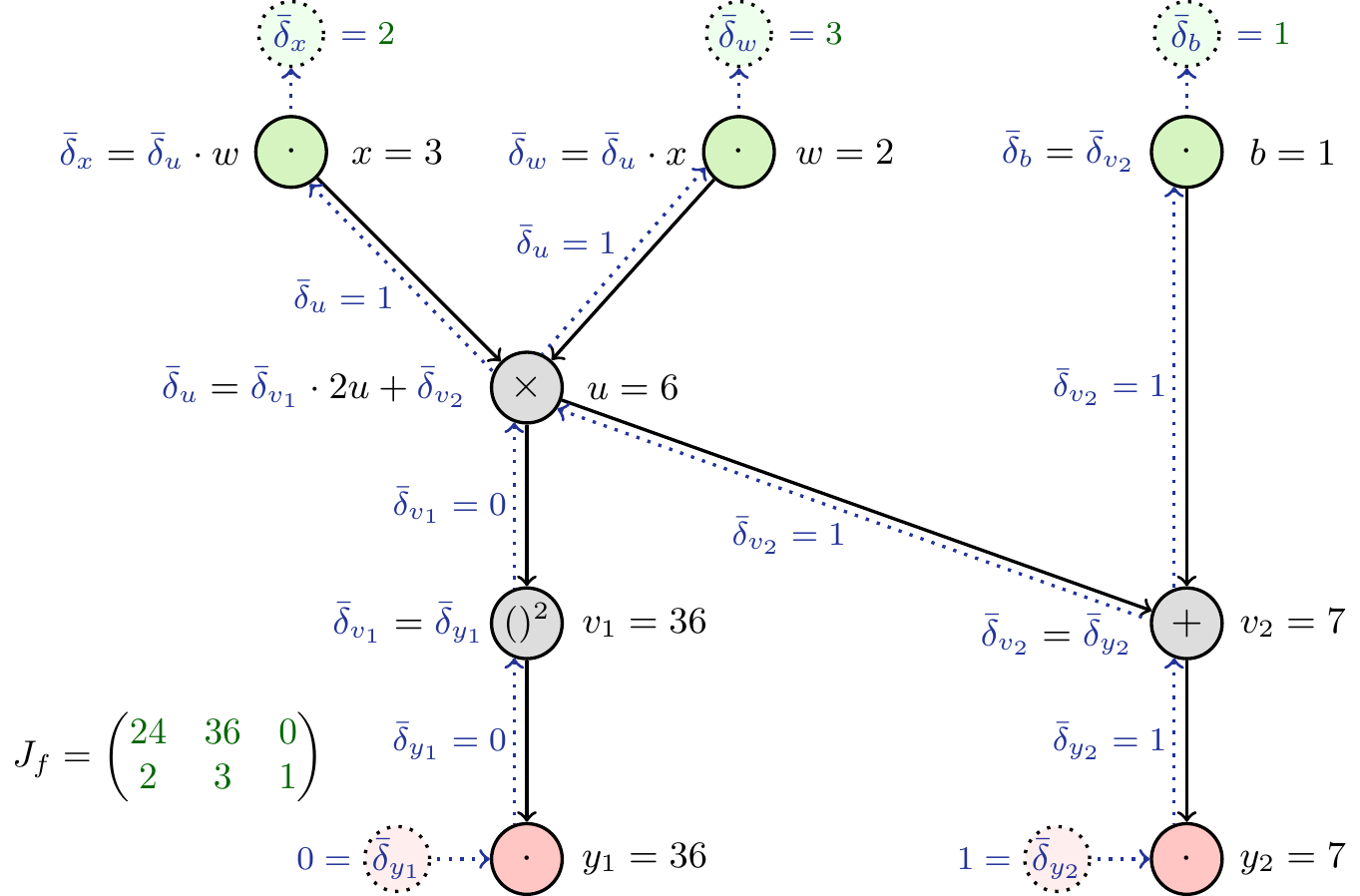
Takeaways
Consider a function \(f: \mathbb{R}^n\to\mathbb{R}^m\) with \(n\) inputs and \(m\) outputs. As we have seen above, in forward mode \(n\) passes are needed to obtain the full Jacobian. In reverse mode, one forward pass and \(m\) reverse passes are needed. Which mode should be used in practice therefore depends on \(n\) and \(m\). If \(n \ll m\), i.e. the function has few inputs and many outputs, forward mode differentiation is usually more efficient. If \(n \gg m\), i.e. the function has many inputs and only few outputs, reverse mode differentiation will be more efficient. The setting encountered in machine learning is an extreme form of the latter, with only one output (the loss) and inputs that can well be in the millions (the parameters). Therefore at least in classical machine learning, reverse mode is exclusively used.
Now we have them all. The principles of Automatic Differentiation. At least in theory.
You might however be interested in applying them to your own source code. How do you actually program differentiably?
Implementation on dynamic code
This section aims to explain the key design principles that form what you can do and how you do it in different automatic differentiation frameworks. You could implement AD from scratch or let one of the mature libraries do the heavy lifting. These libraries – PyTorch, Tensorflow, Jax, Flux.jl – all do the following three things
- take source code that satisfies some requirements for the framework
- build a computational graph for automatic differentiation
- offload compute-heavy operations to fast kernels (often in a low level language)
All libraries make different tradeoffs in how the computational graph is constructed, represented and optimized. Rackauckas (2021) is a great reference for this.
Why is there so much room for choice in the treatment of computational graphs? Well, we have so far neglected that algorithms do not only contain mathematical operations, but also if-branches, for and while-loops. Those dynamic features of code are called control flow.
Tape-based dynamic graph generation
To have a well defined computational graph of the program that we seek to differentiate for a given input, despite the dynamic control flow of the computation, we can record the graph for each input separately. This is called tape-based graph generation to emphasize the live recording. The graph is then thrown away after differentiation.
For each input
- record the atomic operations inside the program when executing it,
- automatically differentiate on the per-input graph,
- and throw away the graph.
The upside is, that we can differentiate arbitrarily dynamic code! Just use the regular control flow statements. This flexibility however comes at the cost of having to recompute the graph for each input.
Purely tape-based AD in PyTorch
import torch

1x = torch.tensor(2.0, requires_grad=True)

def f_torch(x):
    print("calculating f(x)")
    for i in range(3):
2        x = torch.sin(2*x) + x**2
    return x

y = f_torch(x)
y- 1
-
Use PyTorch’s datatype
Tensor;requires_grad=Truetells PyTorch to record the operations onxto build a dynamic computational graph. - 2
-
PyTorch (re)defines the operations
torch.sin,+,*and**to record the operations onxwhen executing any of them.
calculating f(x)
tensor(115.4449, grad_fn=<AddBackward0>)
Now, we instruct PyTorch to do a backward pass according to the reverse mode Automatic Differentiation algorithm. As a result, the gradient of y with respect to x is saved as an attribute of the object x.
y.backward()

x.gradtensor(448.8119)Static graph generation
Using throw-away graphs like above can significantly slow down your program. We can get more performance by avoiding to regenerate a new graph and optimize the graph itself.
How is such a reusable static graph represented and optimized? At first, this will be a bit technical, but it will be worth it when we get to examples soon. Essentially, when the structure of the graph is known in advance, it can be optimized. To make optimal use of this, a static graph is typically
- defined in a high level language,
- compiled from the source code to intermediate representations (IRs) like XLA and LLVM IR, and transformed to include computations of gradients by AD, before it is
- further compiled to machine code for a target machine.
In the Intermediate Representation (IR), the graph is optimized, e.g. by fusing operators together to reduce the memory transfer and kernel launch overhead. See Snider and Liang (2023) for a technical explaination and analysis of the benefits of Operator Fusion. The optimized (compiled) representation is cashed and subsequent calls will reuse the cached graph.
These programs however cannot contain arbitrary control flow. In order to get reusable compiled graphs only a static sublanguage can be used. That excludes regular if, for and while.
Tensorflow originally followed this scheme precisely. When Tensorflow was developed in its first versions (1.x), it relied on specifying a computational graph upfront and separately from the rest of the source code. Since this graph was not dynamically generated, it could be reused for all inputs and optimized for the hardware it would run on. However, having to specify the graph separately from the rest of the program is not very user-friendly – and it puts up strict requirements as it needs the full computation to be static.
For this reason, Tensorflow 1.x is not used anymore. With 2.0 a new mode of operation was introduced, called eager execution, which is essentially the same as PyTorch’s tape-based approach. Both frameworks now converged on the following compromise: For convenience you can tape throw-away graphs, but to be able to do optimization on reusable (sub)graphs you may mark parts of your code to be traced (and compiled) to a static representation.
In Tensorflow this is done by decorating a function with @tf.function. The first time the function is called, the graph is generated and cached. Subsequent calls will reuse the cached graph.
In PyTorch you would use the decorators @torch.jit.script (allows some control flow) or @torch.jit.trace (no control-flow).
We will look at two code examples of static graphs: static subgraphs in Tensorflow 2 and full XLA-based optimization with JAX.
Static subgraph inside a dynamic graph – Tensorflow 2
Let’s take a look! The tf.GradientTape environment is – as the name already hints at – just a different style of tape-based dynamic graph generation. The operation f_tf(x) however is not dynamically traced, since it is decorated with @tf.function.
import tensorflow as tf
import sys

x = tf.Variable(2.0)

1@tf.function
def f_tf(x):
    #this will only be printed once
    print("Hello Python! \
2      (a static graph is created at this first execution)")
    return tf.sin(2*x) + x**2

3with tf.GradientTape(persistent=True) as tape:
    tape.watch(x)
    y = f_tf(x)

dy = tape.gradient(y, x)
print(dy)

x = tf.Variable(3.0)

with tf.GradientTape(persistent=True) as tape:
    tape.watch(x)
4    y = f_tf(x)

dy = tape.gradient(y, x)
print(dy)- 1
- mark the following function as a static graph function
- 2
- this will only be printed once, when the graph is constructed
- 3
-
tf.GradientTaperecords the gradients - 4
- “Hello Python! …” will not be printed again
Hello Python!       (a static graph is created at this first execution)
tf.Tensor(2.6927128, shape=(), dtype=float32)
tf.Tensor(7.9203405, shape=(), dtype=float32)
The print statement does not appear in the cached graph representation. That it is not executed for the second pass is evidence that Tensorflow used a static graph instead of retracing the atomic operations inside f_tf(x).
So this is how you speed up Tensorflow’s eager-execution (i.e. tape-based) Automatic Differentiation, by telling it which subprograms can be represented by reusable static graphs. If your code runs on a GPU, you can replace @tf.function by @tf.function(jit_compile=True) to enable XLA-based optimization like operator fusion.
Here we will look at the JAX-way to XLA-based optimization.
Compiled graphs – XLA in JAX
JAX is built to compile and run NumPy programs. It adopts a functional programming paradigm instead of an object oriented one like PyTorch and Tensorflow. Because functions (methods) in object-oriented programs often have side effects like changing a hidden object state, they are difficult to analyse as a graph. In contrast, functional programs can be thought of as a tree of expressions!
This tree is already close to the computational graph that we are interested in. Thus, we can rely on source code transformation as opposed to operator overloading for the implementation of automatic differentiation.
Source code transformation entails taking the original code and systematically rewriting it into a new form that includes the necessary operations for computing derivatives, as opposed to operator overloading where the standard arithmetic operations are redefined to inject code that records the computation graph.
As we have done with the other frameworks, we define a function f_jax(x) first. JAX provides a function jax.grad that is provided with a function as input and creates a function that is the derivative of the input function. We evaluate it to get the derivative at x = 2.0.
import jax
x = 2.0                 # regular Python float
def f_jax(x):
    for i in range(2):
        x = jax.numpy.sin(2*x) + x**2
    return x

jax.grad(f_jax)(x)
DeviceArray(22.740614, dtype=float32, weak_type=True)
WARNING:jax._src.lib.xla_bridge:No GPU/TPU found, falling back to CPU. (Set TF_CPP_MIN_LOG_LEVEL=0 and rerun for more info.)We can take a look at a the intermediate representations of f_jax: First the so called Jaxpr – short for JAX-representation, then the High-Level Optimizer XLA representation.
jax.make_jaxpr(f_jax)(x){ lambda ; a:f32[]. let
b:f32[] = mul 2.0 a
c:f32[] = sin b
d:f32[] = integer_pow[y=2] a
e:f32[] = add c d
f:f32[] = mul 2.0 e
g:f32[] = sin f
h:f32[] = integer_pow[y=2] e
i:f32[] = add g h
in (i,) }xla_comp = jax.xla_computation(jax.grad(f_jax))(x)
print(xla_comp.as_hlo_text())HloModule xla_computation_f_jax, entry_computation_layout={(f32[])->(f32[])}
ENTRY main.19 {
Arg_0.1 = f32[] parameter(0)
constant.2 = f32[] constant(2)
multiply.3 = f32[] multiply(Arg_0.1, constant.2)
sine.4 = f32[] sine(multiply.3)
multiply.6 = f32[] multiply(Arg_0.1, Arg_0.1)
add.8 = f32[] add(sine.4, multiply.6)
multiply.11 = f32[] multiply(add.8, constant.2)
multiply.9 = f32[] multiply(add.8, constant.2)
cosine.10 = f32[] cosine(multiply.9)
multiply.12 = f32[] multiply(cosine.10, constant.2)
add.13 = f32[] add(multiply.11, multiply.12)
multiply.7 = f32[] multiply(Arg_0.1, constant.2)
multiply.14 = f32[] multiply(add.13, multiply.7)
cosine.5 = f32[] cosine(multiply.3)
multiply.15 = f32[] multiply(add.13, cosine.5)
multiply.16 = f32[] multiply(multiply.15, constant.2)
add.17 = f32[] add(multiply.14, multiply.16)
ROOT tuple.18 = (f32[]) tuple(add.17)
}Notice, that JAX treats the control flow in the function f_jax(x) by unrolling the loop. In the jaxpr, there is no for-loop left, so it handles for loops well.
We can measure how long it takes to calculate the gradient with timeit 1.
from timeit import timeit

f"{timeit(lambda: jax.grad(f_jax)(x), number=100):.5f} seconds"
'0.34105 seconds'To make efficient use of the representations, JAX allows you to just-in-time compile a function by calling jit() on it.
grad_f_jax_jit = jax.jit(jax.grad(f_jax))

grad_f_jax_jit(x).block_until_ready()   # let it trace
DeviceArray(22.740614, dtype=float32, weak_type=True)f"{timeit(lambda: grad_f_jax_jit(x).block_until_ready(), number=100):.5f} seconds"'0.00024 seconds'From a fifth of a second to less than a millisecond! We can see that the runtime can be orders of magnitude faster when using compiled operations. 2
Source-to-source transformation
We have looked at two ways to treat the dynamic nature of programs:
- Allow full flexibility, but pay the price of re-tracing the graph for every input, or
- allow only a subset of possible programs, but gain the ability to reuse the graph.
There is a third way: source to source transformation. In a sense this goes a step further in the direction of what we have seen JAX can do. But instead of transforming a static intermediate representation (like Jaxpr or XLA) to include computations that track the operations and their inputs for AD, we can transform the source code itself.
The trick is to realize, that the structure of the program is static, while the choices made during computation are dynamic. Source-to-source transformation is in the business of figuring out how to transform the code to note and save, for example, how many times some loop was executed during the forward pass. This way, when it comes to the backward pass, this information is still available and the gradients can be pulled back through code including control flow.
So just like tape-based dynamic graph generation, see the first example Section 5.1.1, source-to-source transformation AD also allows arbitrary control flow. The crucial difference however is, that in the former you build one totally separate graph for every input and in the latter you can make it really efficient by doing compiler optimizations on the whole dynamic computation.
So why is not everybody using source-to-source transformation to do differentiable programming if it is so powerful?
It appears to be very difficult to implement this in Python. Python is interpreted instead of being compiled and has many features that emphasize flexibility (like being dynamically typed, not requiring declarations, …). This makes the task to find a source-to-source transformation in Python very challenging 3. In contrast, languages like Julia and Swift have more predictable dynamic behavior, for example they are type-stable, so figuring out how to track the dynamic choices of the full language becomes easier.
Let us take a look at how to differentiate a dynamic regular Julia function with Flux. Flux is the Julia package for machine learning and by default uses the Zygote package in the background for doing source-to-source AD.
using Flux

function f_flux(x)
    # repeat until x is larger than 5, but at most 3 times
    i = 0
    while x < 5 && i < 3
        i += 1
        x = sin(2*x) + x^2
    end
    return x
end
f_flux (generic function with 1 method)
It is impossible to know how often the while-loop will run without specifying an input and doing the computations. Still this framework allows to transform the source code to keep track of the gradients. In the previously discussed frameworks that output compiled graphs, we could not differentiate this!
What does Flux’s higher-order function gradient do if we call it on f_flux?
df(x) = gradient(f_flux, x)df (generic function with 1 method)
With source-to-source transformation we obtained a function df(x) as a general derivative of f_flux for any input.
df(2.0)(22.7406128502423,)
And the original function f_flux was regular Julia code with irreducible control flow! gradient seperates the unknown dynamic choices (how often the loop runs) from the static structure and returns a function optimized on the static structure but still flexible for its dynamic adaptation.
This concludes our tour through the design principles and frameworks of automatic differentiation.
References
Boomgaard, Rein van den. 2021. “Computational Graphs and the Chain Rule of Differentiation.” https://staff.fnwi.uva.nl/r.vandenboomgaard/MachineLearning/LectureNotes/Math/automatic_differentiation.html.
Grosse, Roger. 2018. “Automatic Differentiation.” https://www.cs.toronto.edu/~rgrosse/courses/csc321_2018/slides/lec10.pdf.
Heinrich, Lukas. 2020. “Tutorial on Automatic Differentiation.” https://theoryandpractice.org/stats-ds-book/autodiff-tutorial.html.
Johnson, Matthew James. 2017. “Automatic Differentiation.” http://videolectures.net/deeplearning2017_johnson_automatic_differentiation/.
Rackauckas, Christopher. 2021. “Engineering Trade-Offs in Automatic Differentiation.” https://www.stochasticlifestyle.com/engineering-trade-offs-in-automatic-differentiation-from-tensorflow-and-pytorch-to-jax-and-julia/.
Schiendorfer, Alexander. 2020. “Automatic Differentiation for Deep Learning, by Example.” https://alexander-schiendorfer.github.io/2020/02/16/automatic-differentiation.html.
Snider, Daniel, and Ruofan Liang. 2023. “Operator Fusion in XLA.” http://arxiv.org/abs/2301.13062.
TensorFlow. 2022. “Introduction to Gradients and Automatic Differentiation.” https://www.tensorflow.org/guide/autodiff.
Xu, Kailai. 2020. “What Is ADCME? Computational Graph, Automatic Differentiation & TensorFlow.” https://docs.juliahub.com/ADCME/b8Ld2/0.7.3/tu_whatis/.
Footnotes
If you have access to IPython, use the magic command
%timeit. Quarto currently doesn’t support IPython magic and latex rendering in the same document.↩︎Remember, that PyTorch and Tensorflow in principle also allow you to compile parts of the differentiable program as shown in the Tensorflow example, Section 5.2.1. But JAX is really focused on specifically this.↩︎
But it has been tried. See the (abandoned) Tangent repo: https://github.com/google/tangent.↩︎