Ensembles of neural networks helps us understand learner variability.
From a perspective of Bayesian updating, the training dataset does not uniquely identify a single trained neural network, rather it constrains the high-dimensional parameter space. Many approaches to Bayesian neural networks adapt the neural architecture in an attempt to approximate a distribution over trained neural networks, but among the most straightforward approaches – thus appealing, albeit costly – is the ensemble.
As is common in simulation-based inference, we will consider a network that consists of
a summary network – an embedding learner that produces fixed length vectors by compressing a more complex data modality, and
an inference network – a conditional generative network which takes the embeddings as input condition and produces samples from a target distribution.
Specifically, we will learn the posterior over model parameters given the observations as conditions, also called amortized neural posterior estimation (NPE).
The idea I want to explore in this post is to have a shared summary network for an ensemble of inference networks. Sharing the summary network is more efficient than learning multiple in the same way that learning just a single inference network would be cheaper than multiple. But the reasonable hope is, that many of the benefits of ensembles are already unlocked by duplicating just the final part of the network. The argument for this kind of “last-part-of-network-ensemble” parallels that of last-layer-Bayesian neural networks.
So in this blog post I am sharing an implementation of an ensemble of conditional generative models (just below) and we will try it out on a classic Bayesian parameter estimation task: Lotka-Volterra predator prey dynamics.
Show general imports
%load_ext autoreload%autoreload 2import osos.environ["KERAS_BACKEND"] ="jax"import numpy as npimport bayesflow as bfimport matplotlib.pyplot as pltimport seaborn as snsimport scipyfrom scipy.integrate import odeint
This class is designed to be a drop in replacement for inference networks in BayesFlow. To construct an instance, we pass a dictionary of BayesFlow inference networks, which will be the ensemble members. The class channels input and output to and from each of the essential inference network methods to allow parallel training and estimation: * compute_metrics : includes loss computation for training with stochastic gradient decent * sample & log_prob : sample from and evaluate the learnt conditional distribution
As you can see in the code, it works by looping over ensemble members and delegating to their respective methods.
The ensemble above wraps inference networks, but in fact is itself a drop in replacement to conventional BayesFlow inference networks. Instead of using just one coupling flow, we get two which are identical except for their initialization and a flow matching model on top of that.
It will be interesting to see how the three models behave differently and we will give them a spin on Lotka-Volterra.
Example: Lotka-Volterra parameter estimation from time series
Suppose we measured population counts from two species over time. One of them preys on the other, so we might assume that the dynamics are governed by the classic Lotka-Volterra system. In dimensionless form, with prey population \(x\) and predator population \(y\), the nonlinear differential equation is
As always, this model entails a number of assumptions that can only be approximate reality. In brief: On their own, prey count increases exponentially with rate \(\alpha\), while predator count decays with rate \(\gamma\). Interesting dynamics are possible when both predators and prey are present: The number of predators increases the more prey it can hunt, reducing prey counts proportionally at a rate \(\beta\) and increasing predator count proportionally at a rate \(\delta\).
We can measure population timeseries, but never the parameters directly, so this is a scientifically relevant inverse problem.
Our simulator will consist of three parts:
First, we choose a prior distribution over parameters that reflects our beliefs about parameters before observing data.
Building on parameters sampled from the prior, we solve the parameterized Lotka-Volterra equation starting from some initial conditions.
Finally, we hypothesize that we will make some counting errors when observing the populations, introducing a Gaussian error on the true populations.
Show implementation of Lotka-Volterra observation model
rng = np.random.default_rng(seed=1234)def prior(): x = rng.normal(size=4) theta =1/(1+np.exp(-x)) *3.9+0.1# logit normal distribution scaled to range from 0.1 and 4returndict( alpha=theta[0], beta=theta[1], gamma=theta[2], delta=theta[3], )def lotka_volterra_equations(state, t, alpha, beta, gamma, delta): x, y = state dxdt = alpha * x - beta * x * y dydt =- gamma * y + delta * x * yreturn [dxdt, dydt]def ecology_model(alpha, beta, gamma, delta, t_span=[0, 5], t_steps=100, initial_state=[1, 1]): t = np.linspace(t_span[0], t_span[1], t_steps) state = odeint(lotka_volterra_equations, initial_state, t, args=(alpha, beta, gamma, delta)) x, y = state.T # Transpose to get x and y arraysreturndict( x=x, # Prey time series y=y, # Predator time series t=t, # time )def observation_model(x, y, t, subsample=10, obs_prob=1.0, noise_scale=0.1): t_steps = x.shape[0]# Add Gaussian noise to observations noisy_x = rng.normal(x, noise_scale) noisy_y = rng.normal(y, noise_scale)# Determine which time steps are observed step_indices = np.arange(0, t_steps, subsample) num_observed =int(obs_prob *len(step_indices)) observed_indices = np.sort(rng.choice(step_indices, num_observed, replace=False))return {"observed_x": noisy_x[observed_indices],"observed_y": noisy_y[observed_indices],"observed_t": t[observed_indices] }
Adapter for preprocessing simulated data for neural processing
learned_sumstat_adapter = ( bf.adapters.Adapter()# convert any non-arrays to numpy arrays .to_array()# convert from numpy's default float64 to deep learning friendly float32 .convert_dtype("float64", "float32")# drop unobserved full trajectories .drop(["x", "y", "t"])# add a trailing dimension of 1 .as_time_series(["observed_x", "observed_y", "observed_t"])# rename the variables to match the required approximator inputs .concatenate(["alpha", "beta", "gamma", "delta"], into="inference_variables") .concatenate(["observed_x", "observed_y", "observed_t"], into="summary_variables"))learned_sumstat_adapter
… and define the full pipeline of the neural approximation to the conditional distribution parameters given observation.
In this pipeline the heart will be the inference_network_ensemble object that we have defined earlier. Even though it is not a single network but an ensemble of them, the user can conveniently plug it in as an inference network.
approximator = bf.PointApproximator( adapter=learned_sumstat_adapter, summary_network=bf.networks.TimeSeriesNetwork(), inference_network=inference_network_ensemble, # THIS IS AN ENSEMBLE OF INFERENCE NETWORKS)total_steps =int(epochs * num_batches)warmup_steps =int(0.05* epochs * num_batches)decay_steps = total_steps - warmup_stepslearning_rate = keras.optimizers.schedules.CosineDecay( initial_learning_rate=0.1*5e-4, warmup_target=5e-4, warmup_steps=warmup_steps, decay_steps=decay_steps, alpha=0,)optimizer = keras.optimizers.Adam(learning_rate, clipnorm=1.5)approximator.compile(optimizer=optimizer, metrics=None)
history = approximator.fit(dataset=dataset, epochs=epochs, verbose=0, validation_data=learned_sumstat_adapter(val_sims))
INFO:bayesflow:Fitting on dataset instance of OfflineDataset.
INFO:bayesflow:Building on a test batch.
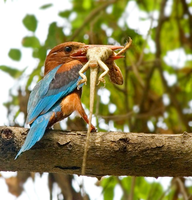
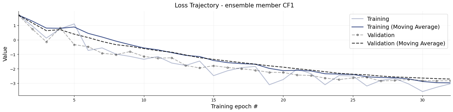
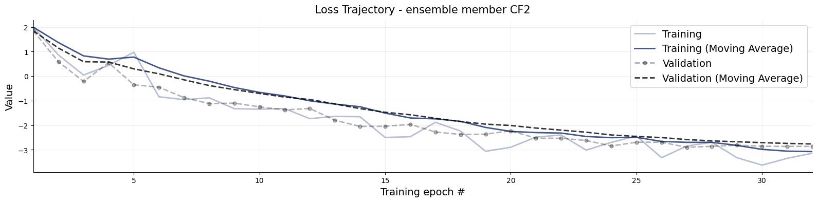
title_args =dict(y=1.02, size=15)for k,v in inference_network_ensemble.networks.items(): f = bf.diagnostics.loss(history, train_key=f"{k}/loss/inference_{k}/loss", val_key=f"val_{k}/loss/inference_{k}/loss") f.gca().set_title(f"Loss Trajectory - ensemble member {k.upper()}", **title_args)
The loss curves are how we like them. Monotonically falling and without significant differerence of performance on training (solid line) and validation dataset (dashed line).
The first interesting thing we observe is, that the two Coupling Flows (CF1 & CF2) have quite similar loss fluctuations. Remember, they only differ by their initialization, but always recieve the same training batches across training. So we notice that equal training batches are performing similarly regardless with differing initializations not manifesting much differences in loss. Both networks see the same loss landscape and likely stay close for that reason. Still, they start at different positions and stay at different postitions.
From a dynamical systems perspective, we can think of training a neural network for an epoch as an iterative map and study whether that map is chaotic.1 So what we are seeing is that if we consider the loss on the same data as an indicator for similarity/discrepancy and infer some metric from that, the training is not chaotic here.
NOTE: I spoke to the the discrepancy of the two coupling flows but not to the different architecture, Flow Matching. This is for good reason: Their losses measure something different and cannot be straightforwardly compared.
We will now assess the discrepancy of the learnt distributions. First, we can sample from the trained approximator object just like any other BayesFlow object.
%%time# Set the number of posterior draws you want to getnum_samples =500# Obtain posterior draws with the sample methodpost_draws = approximator.sample(conditions=val_sims, num_samples=num_samples)# post_draws is a dictionary of draws with one element per named parameterspost_draws.keys()
CPU times: user 8min 54s, sys: 14.5 s, total: 9min 8s
Wall time: 1min 15s
dict_keys(['cf1', 'cf2', 'fm1'])
The only difference is that posterior draws will be a nested dictionary where first level key-values pairs correspond to sample for the different ensemble members (inference networks).
Let’s move on and look at the recovery, calibration and an examplary posterior distribution for each ensemble member.
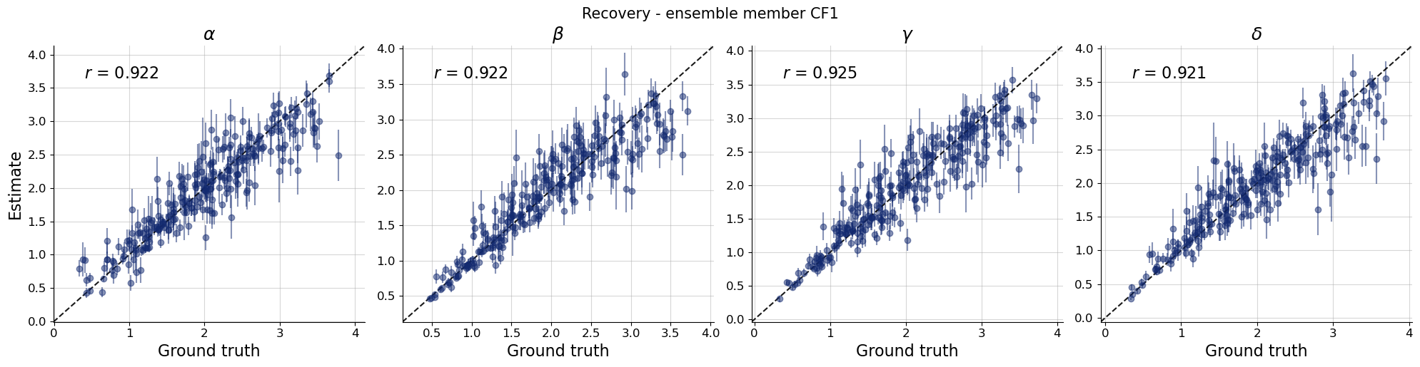
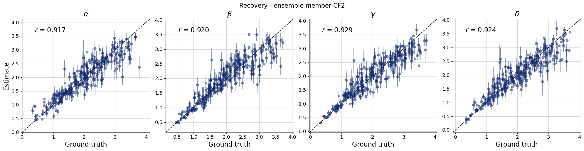
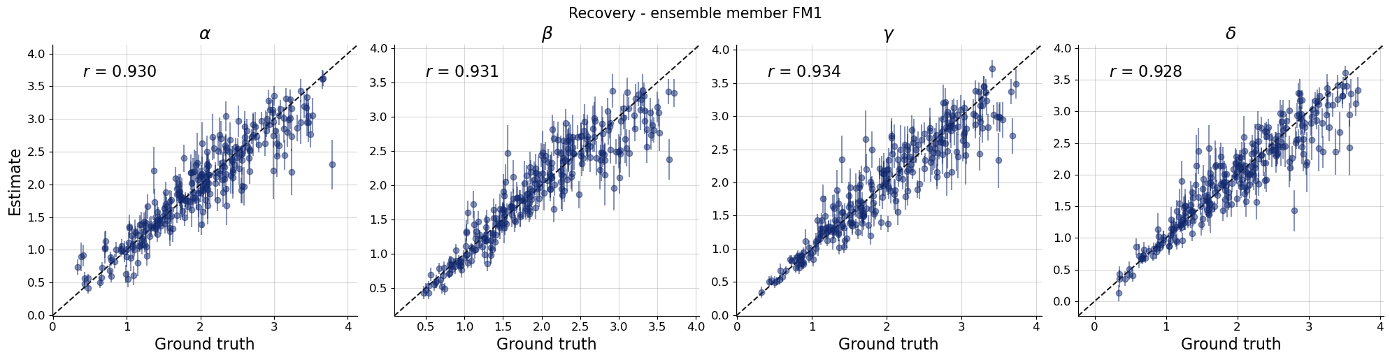
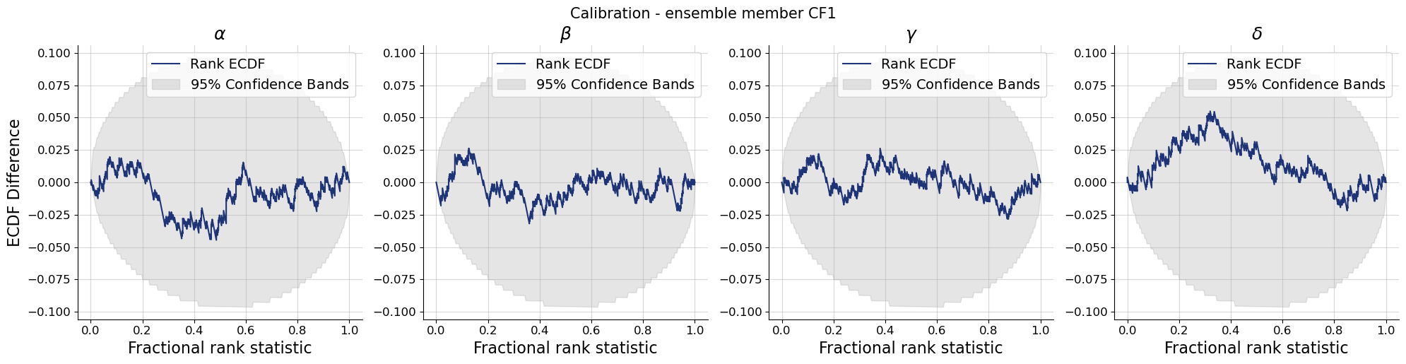
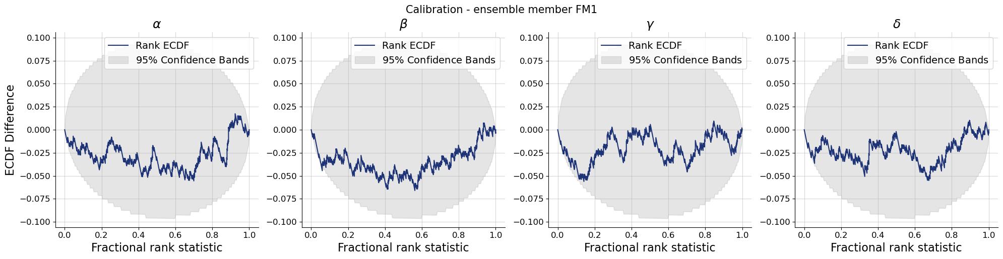
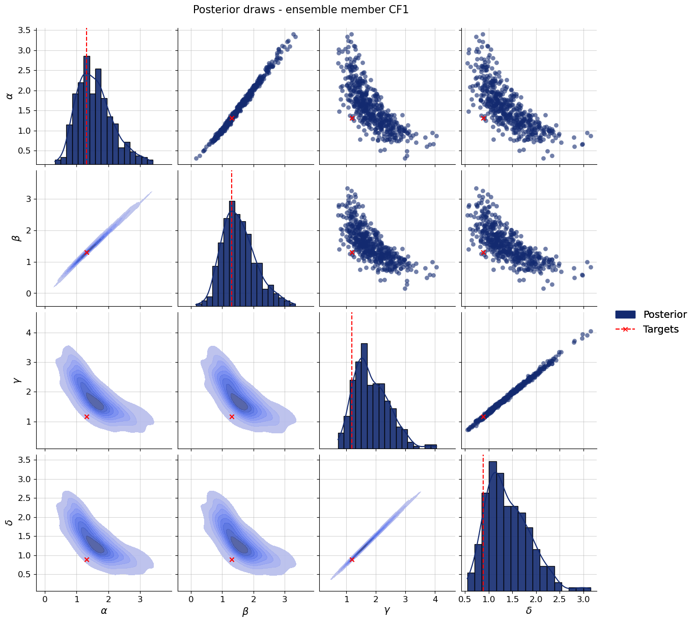
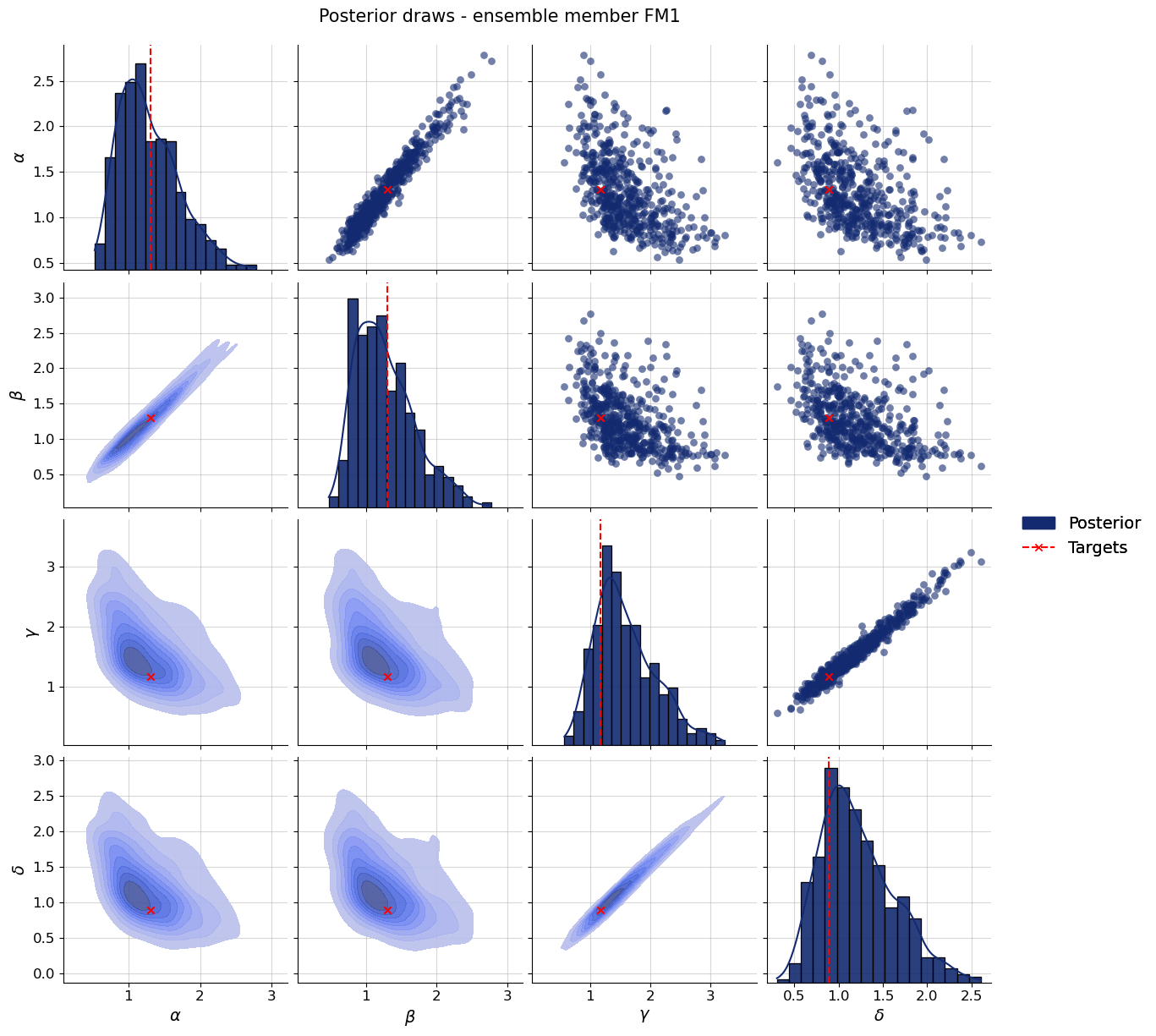
par_names = [r"$\alpha$", r"$\beta$", r"$\gamma$", r"$\delta$"]dataset_id =0for k,v in post_draws.items(): f = bf.diagnostics.recovery(v, val_sims, variable_names=par_names) f.suptitle(f"Recovery - ensemble member {k.upper()}", **title_args)for k,v in post_draws.items(): f = bf.diagnostics.calibration_ecdf(v, val_sims, variable_names=par_names, difference=True) f.suptitle(f"Calibration - ensemble member {k.upper()}", **title_args)for k,v in post_draws.items(): g = bf.diagnostics.plots.pairs_posterior( estimates=post_draws[k], targets=val_sims, dataset_id=dataset_id, variable_names=par_names, ) g.fig.suptitle(f"Posterior draws - ensemble member {k.upper()}", **title_args)
Calibration and recovery look really similar, although not identical, across the board. What stands out most is that Flow Matching posteriors are significantly less contracted.
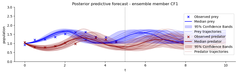
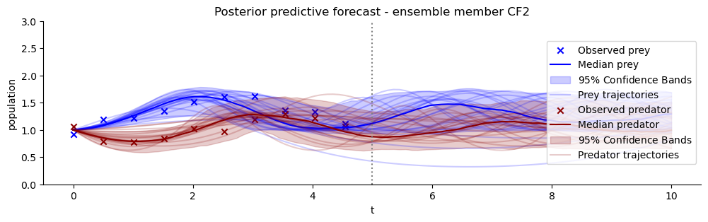
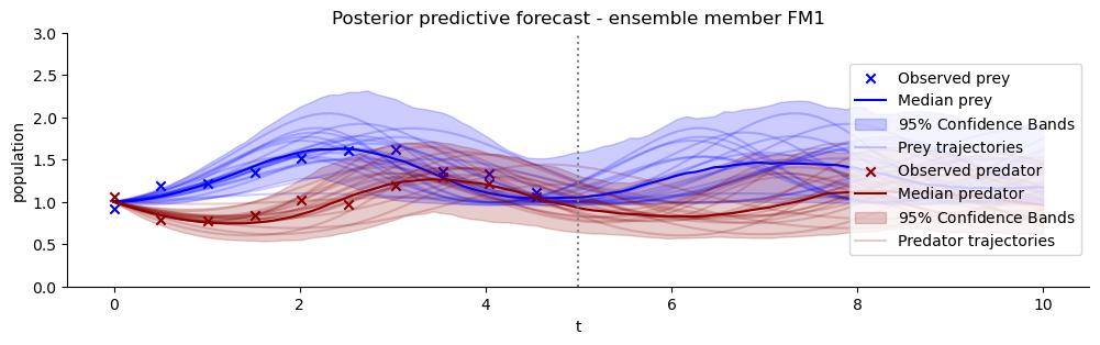
Finally, any good Bayesian inference experiment should check the posterior predictive distributions that the (here: learnt) posteriors result in. We will plot the observation that was used as condition for an examplary posterior and the forecasts of the estimated model – again for each ensemble member.
Even the tiniest difference in initial conditions would blow up eventually if the map was chaotic. Check out the Lyapunov exponent for a precise conceptionalization of chaos.↩︎

