Show imports
import matplotlib.pyplot as plt
import numpy as np
import pandas as pd
import seaborn as sns
import collections
import scipy

RNG = np.random.default_rng(1111)Can we explicitly invert models?
In science, models are developed to explain 1 data.
\[x \sim \mathcal{M}(\theta)\]
To use measured data to explain 2 models we often need to solve the inverse problem. \[\theta \sim \mathcal{M}^{-1}(x)\]
This is hard, because
Simulation-based inference (SBI) methods seek to solve this inverse problem for any black-box simulator, see e.g. Cranmer, Brehmer, and Louppe (2020), (radev2022?). Usually, the simulator is actually known in detail as source code, but we shy away from using that knowledge and thus treat it as a black box!
How far can we actually get with inverting the simulator explicitly?
We will look at an example where we succeed and efficiently acquire exact samples of the true posterior, without any approximation.
The goal will be to find the set of all solutions \(\theta\) of \(\mathcal{M}(\theta) = x\) and the probability of those solutions.
Inverting the simulator comes down to solving a system of equations, if the simulator has no internal randomness. In fact, for this method to work, we need a deterministic formulation of the simulator to move forward. Often, when a simulator involves sampling from a distribution, like for example additive noise, we can reparametrize to get an explicit noise dependence and treat the noise variables as parameters.
\[x \sim \mathcal{M}(\theta) \quad \rightarrow \quad x = \mathcal{M}(\theta, \xi)\]
Externalize the randomness! Drawing \(\xi \sim p(\xi|\theta)\) we get the stochasticity of \(x\) again.
Now, going backward through the simulator code we collect internal state variables \(z\) and equations describing their relation to the known data \(x\) and unknown parameters \(\theta\).
Depending on the model, solving this system of equations is more or less difficult. The result, however, will be an inverse problem with fewer parameters, since it used the model implicit constraints and data constraints. If we are entirely successful, we even get a parametrization of all possible \(\theta_{1...n}\) in terms of a subset \(\theta_{1...k}\).
Then you get exact posterior samples from \(\theta \sim p(\theta|x)\) like so:
A reduced parameterization includes the functional dependency \(f(\theta_{1...k})\) and the applicable set of \(\theta_{1...k}\) values. If the bounds of the applicable are not explicitly available, we can always propose from the prior (step 2) and reject if the individual sample is not applicable for the parametrization of \(\theta_{k+1...n}\).
Further, to weigh the resulting solutions according to the prior (step 4) we have at least two options. One is rejecting each sample with a probability proportional to the prior. Another is recording the probability as a weight for each sample, i.e. importance sampling. The first is more straightforward for downstream use since it gives us equal-weight samples, while the second is more sample efficient since it retains all samples even in low-density areas.
Some distributions are implicitly defined. This means we can only sample from them, but not evaluate the density. If we find parametrizations such that the dependant parameters \(\theta_{k+1...n}\) are the ones where we can evaluate the density we make even these difficult simulators tractable!
A community benchmark proposed in Kruse et al. (2021) for simulation-based inference is to find the distribution of robot arm configurations that end in a specified location.
Our robot arm with one rail and three joints is defined by four variables. \(\theta_1\) is the vertical displacement on the robot’s rail system. \(\theta_2, \theta_3, \theta_4\) are angles of the joints. After each joint, there is an arm segment of some length \(l\). At the end of the arm, the so-called end effector can interact with the environment.
\[ \vec x = \begin{bmatrix} 0 \\ \theta_1 \end{bmatrix} + l_2 \begin{bmatrix} \cos (\theta_2) \\ \sin( \theta_2) \end{bmatrix} + l_3 \begin{bmatrix} \cos (\theta_2+\theta_3) \\ \sin( \theta_2+\theta_3) \end{bmatrix} + l_4 \begin{bmatrix} \cos (\theta_2+\theta_3+\theta_4) \\ \sin( \theta_2+\theta_3+\theta_4) \end{bmatrix} \]
The geometry together with a robot’s configuration given by \(\theta\) defines a unique position of the end effector, shown below as a red dot:
import matplotlib.pyplot as plt
import numpy as np
import pandas as pd
import seaborn as sns
import collections
import scipy
RNG = np.random.default_rng(1111)def robot(theta, l=[1, 1, 1], return_all=False):
l2, l3, l4 = l
theta1, theta2, theta3, theta4 = theta
z1 = np.array([0, theta1])
z2 = z1 + l2 * np.array([np.cos(theta2),
np.sin(theta2)])
z3 = z2 + l3 * np.array([np.cos(theta2 + theta3),
np.sin(theta2 + theta3)])
z4 = z3 + l4 * np.array([np.cos(theta2 + theta3 + theta4),
np.sin(theta2 + theta3 + theta4)])
if return_all:
return np.array([z1, z2, z3, z4])
return z4plot_robot()def robot_figure(ax=None, clean=False):
if ax is None:
fig, ax = plt.subplots(figsize=(6, 6))
# Plot the robot arm
ax.vlines(0, -1, 1, color='lightgrey', linewidth=2)
ax.set_ylim([-1.1, 1.1])
ax.set_xlim([-0.1, 2.1])
ax.set_aspect('equal')
if clean:
# Remove border and ticks
ax.spines['top'].set_visible(False)
ax.spines['right'].set_visible(False)
ax.spines['left'].set_visible(False)
ax.spines['bottom'].set_visible(False)
ax.set_xticks([])
ax.set_yticks([])
else:
ax.set_xlabel('$x_1$')
ax.set_ylabel('$x_2$')
return ax
def plot_robot(positions, ax, alpha):
ax.plot(positions[:, 0], positions[:, 1], 'o-', color='grey', markersize=2, alpha=alpha)
ax.plot(positions[0, 0], positions[0, 1], linewidth=5, color='grey', marker='s', markersize=5, alpha=alpha)
ax.plot(positions[-1, 0], positions[-1, 1], linewidth=5, color='red', markerfacecolor='red', marker='o')l = [0.5, 0.5, 1]
angles = np.array([0.5, 0.1, 0, -0.3])
positions = robot(angles, l, return_all=True)
ax = robot_figure()
plot_robot(positions, ax=ax, alpha=1)
angles = np.array([-0.1, -0.7, 1, -0.3])
positions = robot(angles, l, return_all=True)
plot_robot(positions, ax=ax, alpha=0.5);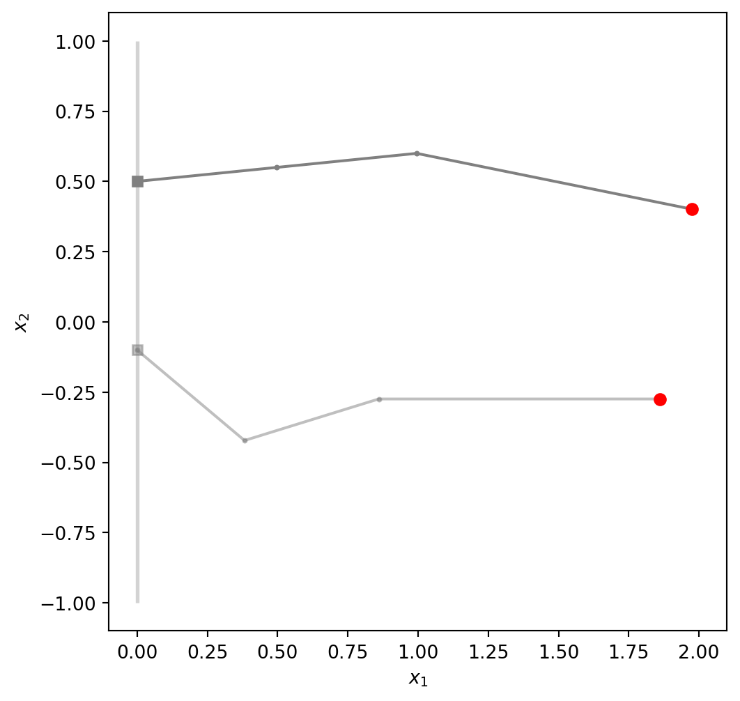
For a given position, only a low-dimensional set of parameters is available. These are solutions of a system of equations.
We leverage that we know the precise relations that together make up \(\vec x=\mathcal{M}(\theta)\). 3 Consider that we have four parameters \(\theta_i\) and two equations for them since \(x\) is two-dimensional. We thus should be able to eliminate two of the parameters. For example, we can express \(\theta_3\) and \(\theta_4\) as functions of \(\theta_1\) and \(\theta_2\). We could use a symbolic solver like sympy or solve the system by hand.
In this case, geometry helps us to solve it by hand. By the forward process, \(\theta_1\) and \(\theta_2\) define a (intermediate, latent) position in real space. \[ \vec z_2 = \begin{bmatrix} 0 \\ \theta_1 \end{bmatrix} + l_2 \begin{bmatrix} \cos \theta_2 \\ \sin \theta_2 \end{bmatrix} \]
The last two segments need to bridge the gap \(| \vec x - \vec z_2 |\), forming a triangle with side lengths \(l_3\), \(l_4\) and \(| \vec x - \vec z_2 |\).
Does this triangle exist? It does, if the triangle inequality is true for all combinations:
\[l_3 + l_4 \gt | \vec x - \vec z_2 |\] \[l_3 + | \vec x - \vec z_2 | \gt l_4\] \[l_4 + | \vec x - \vec z_2 | \gt l_3\]
If such a triangle can exist, then there are exactly two possible solutions. One of them corresponds to joint \(\vec z_3\) being above and the other below the connecting line between \(\vec z_2\) and \(\vec x\). We can use the Law of cosines to determine the correct angles for both cases.
To put this to the test, we can implement functions that
def vec_robot(Theta, l, return_all=False):
    "Determine the position of the joints and the end-effector."
    l2, l3, l4 = l
    Theta_1, Theta_2, Theta_3, Theta_4 = Theta[:, 0], Theta[:, 1], Theta[:, 2], Theta[:, 3]

    Z1 = np.stack([np.zeros_like(Theta_1), Theta_1], axis=1)
    Z2 = Z1 + l2 * np.stack([np.cos(Theta_2),
                             np.sin(Theta_2)], axis=1)
    Z3 = Z2 + l3 * np.stack([np.cos(Theta_2 + Theta_3),
                             np.sin(Theta_2 + Theta_3)], axis=1)
    Z4 = Z3 + l4 * np.stack([np.cos(Theta_2 + Theta_3 + Theta_4),
                             np.sin(Theta_2 + Theta_3 + Theta_4)], axis=1)

    if return_all:
        return np.stack([Z1, Z2, Z3, Z4], axis=1)
    return Z4

def vec_check_reachable(Theta_reduced, X, l):
    "Check if the end effector is in range for a batch of thetas and xs."
    l2, l3, l4 = l
    Theta_1, Theta_2 = Theta_reduced[:, 0], Theta_reduced[:, 1]
    Z1 = np.stack([np.zeros_like(Theta_1), Theta_1], axis=1)
    Z2 = Z1 + l2 * np.stack([np.cos(Theta_2), np.sin(Theta_2)], axis=1)
    h = np.linalg.norm(X - Z2, axis=1)
    c1 = h <= l3 + l4
    c2 = l3 <= h + l4
    c3 = l4 <= h + l3
    return np.all([c1, c2, c3], axis=0)

def vec_get_full_theta(x, Theta_reduced, l):
    "Get the full theta from the reduced theta and end-effector position x."
    l2, l3, l4 = l
    Theta_1, Theta_2 = Theta_reduced[:, 0], Theta_reduced[:, 1]
    Z1 = np.stack([np.zeros_like(Theta_1), Theta_1], axis=1)
    Z2 = Z1 + l2 * np.stack([np.cos(Theta_2), np.sin(Theta_2)], axis=1)
    gap = x - Z2
    eta = np.arcsin(gap[:, 1] / np.linalg.norm(gap, axis=1))
    gamma = np.arccos((l3**2 + np.linalg.norm(gap, axis=1)**2 - l4**2) / (2 * l3 * np.linalg.norm(gap, axis=1)))
    gamma_prime = np.arccos((l4**2 + np.linalg.norm(gap, axis=1)**2 - l3**2) / (2 * l4 * np.linalg.norm(gap, axis=1)))
    theta_3 = -Theta_2 + eta - gamma * np.array([1, -1])[:, None]
    theta_4 = -Theta_2 - theta_3 + eta + gamma_prime * np.array([1, -1])[:, None]
    return np.stack([
                np.stack([Theta_1, Theta_2, theta_3[0,:], theta_4[0,:]], axis=1),
                np.stack([Theta_1, Theta_2, theta_3[1,:], theta_4[1,:]], axis=1)
], axis=1)def pdf_from_distdict(distdict):
"Returns a function that computes the pdf or a single vector."
return lambda x: np.prod([distdict[k].pdf(x[i]) for i, k in enumerate(distdict.keys())])
def vec_pdf_from_distdict(distdict):
"Returns a function that computes the pdfs for rows of a matrix in parallel."
return lambda X: np.prod([distdict[k].pdf(X[:, i]) for i, k in enumerate(distdict.keys())], axis=0)
def sample_from_distdict(distdict, samples=1000):
"Returns a matrix of samples from the distributions in distdict."
return np.array([th.rvs(samples, random_state=RNG) for th in distdict.values()]).T
def slice_distdict(distdict, keys):
return collections.OrderedDict((key, value) for key, value in prior.items()
if key in keys)Now we can put everything together. We fully define the inverse problem by the prior, the lengths of the arm segments, and the end-effector position.
# Define prior, forward process (geometry), and data x (end-effector position)
prior = collections.OrderedDict(
    theta_1 = scipy.stats.norm(0, 0.25),
    theta_2 = scipy.stats.norm(0, 0.5),
    theta_3 = scipy.stats.norm(0, 0.5),
    theta_4 = scipy.stats.norm(0, 0.5),
)

l=[0.5, 0.5, 1]

x = np.array([1.7, 0.2])
We can now apply the steps discussed above:
# Sample theta_1, theta_2 from the prior
n_samples=100_000
reduced_prior = slice_distdict(prior, ['theta_1', 'theta_2'])
complement_prior = slice_distdict(prior, ['theta_3', 'theta_4'])
red_prior_samples = sample_from_distdict(reduced_prior, n_samples)

# Reject samples for which the end effector is not in range
accepted_red_prior_samples = red_prior_samples[vec_check_reachable(red_prior_samples, x, l)]
acc_rate = len(accepted_red_prior_samples) / n_samples
print(f"Acceptance rate from reachability: {acc_rate:.5f}")

# Explicitly calculate preimages theta_3 and theta_4 of x given theta_1, theta_2
theta = vec_get_full_theta(x, accepted_red_prior_samples, l).reshape(-1, 4)

# Weight the samples by their probability under the prior
weights = vec_pdf_from_distdict(complement_prior)(theta[:,2:])
posterior = theta[RNG.binomial(1, weights / np.max(weights))==1]
print(f"Acceptance rate from prior:        {len(posterior) / len(theta):.5f}")
print(f"{len(posterior)} posterior samples from {n_samples} trials")
Acceptance rate from reachability: 0.92158
Acceptance rate from prior: 0.04064
7491 posterior samples from 100000 trialsLet us take a look at the distribution of robot arms now.
# Plot posterior samples
ax = robot_figure(clean=True)
for i, sample in enumerate(posterior[:1000]):
    positions = robot(sample, l, return_all=True)
    plot_robot(positions, ax=ax, alpha=0.05)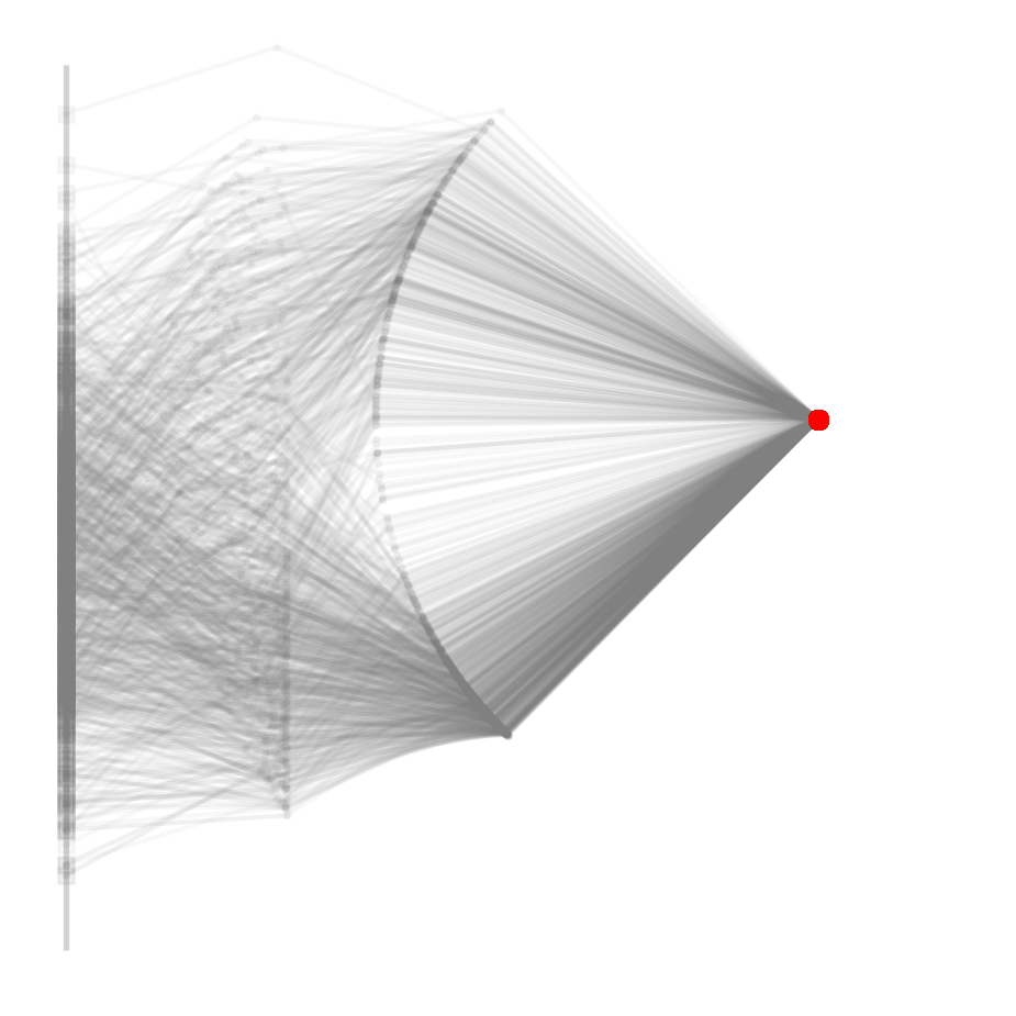
The grid of first order correlations nicely shows the prior distribution (grey), the explicitly calculated solutions (blue), and how they are combined to form a posterior distribution (orange). The parts of the blue solutions distribution that are likely under the grey prior are part of the orange posterior. Also note how the prior enforces a bimodal posterior in \(\theta_2\) (the first joint angle), observable on the second plot on the grid diagonal.
# Plot prior samples and computed Theta in the same pairplot
n_slice = posterior.shape[0]
prior_samples = sample_from_distdict(prior, posterior.shape[0])
param_names = [r'$\theta_1$', r'$\theta_2$', r'$\theta_3$', r'$\theta_4$']
df_prior = pd.DataFrame(prior_samples, columns=param_names).assign(distribution='prior', weights=weights.mean() / np.max(weights))
df_solutions = pd.DataFrame(theta[:n_slice], columns=param_names).assign(distribution='solutions', weights=weights.mean() / np.max(weights)) #weights[:n_slice] / np.max(weights))
df_posterior = pd.DataFrame(posterior, columns=param_names).assign(distribution='posterior', weights=1)
df_both = pd.concat([df_prior, df_solutions, df_posterior])
g = sns.PairGrid(data=df_both[param_names + ['distribution']],
                 hue='distribution', palette=['grey', 'blue', 'orange'], height=2)
g.map_diag(sns.kdeplot, levels=4, bw_adjust=1.2, alpha=0.8, weights=df_both['weights'], common_norm=False)
g.map_lower(sns.scatterplot, alpha=0.5, s=1)
def hide_current_axis(*args, **kwds):
    plt.gca().set_visible(False)
g.map_upper(hide_current_axis)
g.add_legend()
sns.move_legend(g, "center right", bbox_to_anchor=(0.85, .55))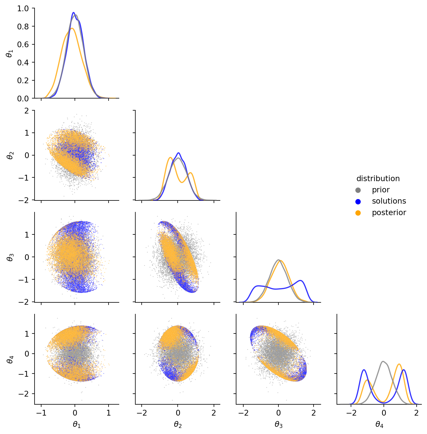
Typically, a newly proposed inference method is validated by measuring the approximation error of its posterior against a reference posterior from a trusted method.
Until now, this trusted method for the inverse-kinematics problem is rejection sampling. Rejection sampling uses brute force, is costly and not exact. However, the appeal remains that it is general and one can directly control the approximation error. This is how it works: Draw four-dimensional robot arm configuration proposals from the prior and reject all but the ones leading to an end-effector position \(x\) close to the desired one.
In our case we do not expect any approximation error at all – the proposed method should result in samples from the exact posterior. However, we should still validate it against the state of the art to rule out bugs and scrutinize whether the method works at all! In fact, before VP did the comparison against rejection sampling I had an undetected bug.
So let us do rejection sampling to reproduce the above posterior.
n_trials = 10_000_000_000
batch_size = 500_000
ref_sample_list = []
for i in range(n_trials//batch_size):
    prior_samples = sample_from_distdict(prior, batch_size)
    x_prior = vec_robot(prior_samples, l=l)
    close_enough = np.linalg.norm(x_prior-x, axis=1) < 0.0005
    ref_sample_list.append(prior_samples[close_enough])
reference_samples = np.concatenate(ref_sample_list)

print(f"{len(reference_samples)} reference posterior samples from {n_trials} trials")

ax = robot_figure(clean=True)
for i, sample in enumerate(reference_samples[:1000]):
    positions = robot(sample, l, return_all=True)
    plot_robot(positions, ax=ax, alpha=0.05)
1042 reference posterior samples from 10000000000 trials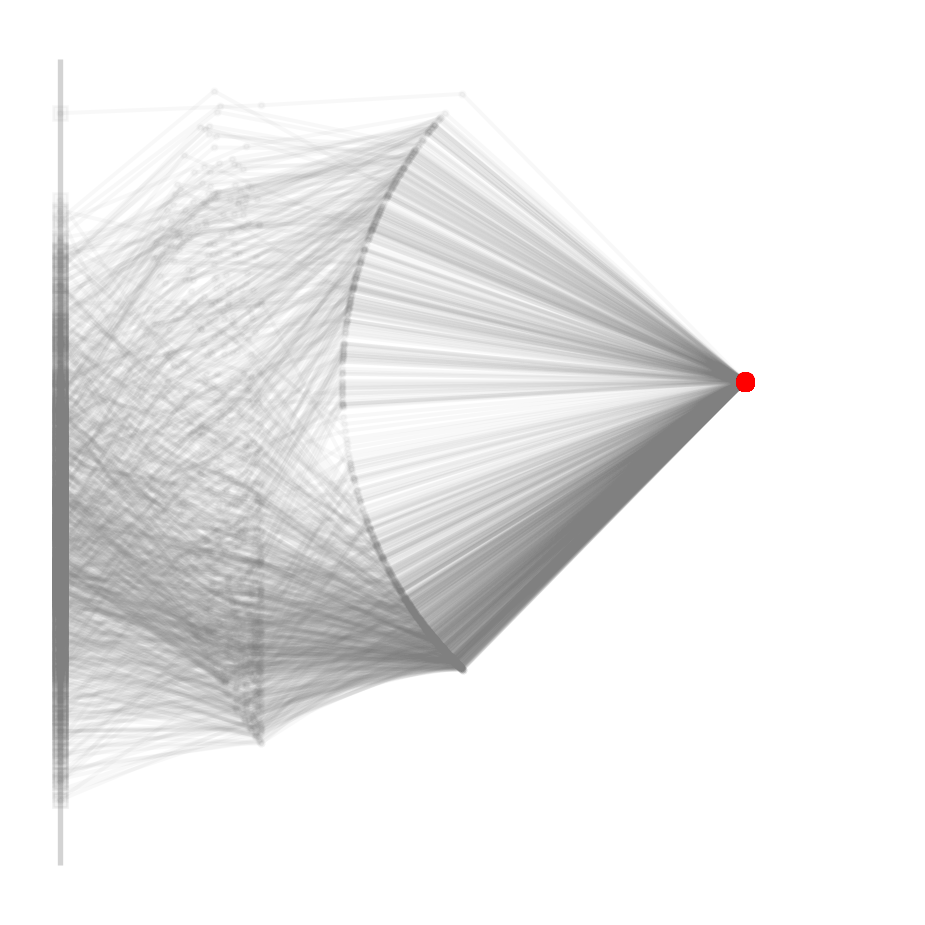
Note that this is not only imprecise, but also used up 100,000 times more proposals, ten billion to be precise. The vast majority gets rejected and we end up with less posterior samples than with the newly proposed method.
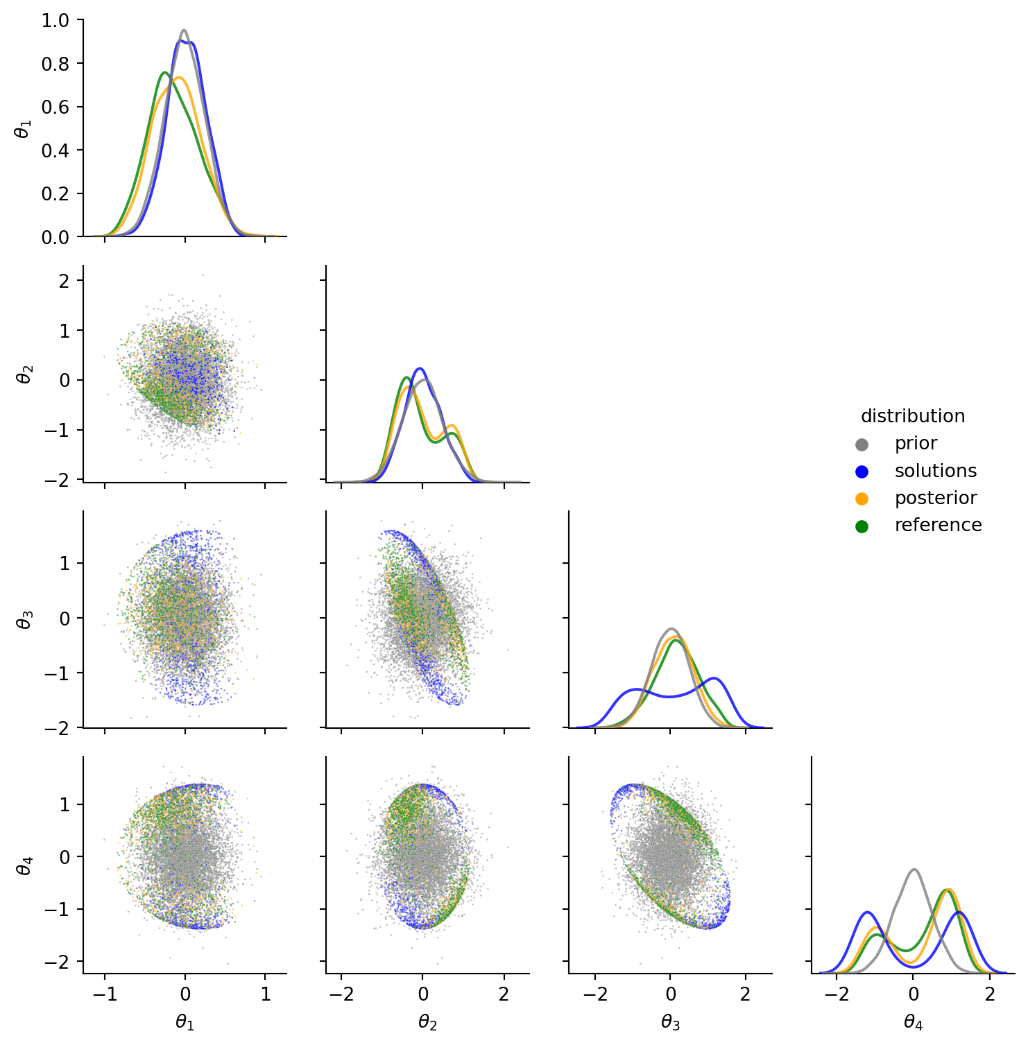
Finally, we can again compare the marginal distributions and pairwise-scatter plots. Orange samples from the newly proposed exact method match well enough with the inexact green reference posterior from rejection sampling.
# Plot prior samples and computed Theta in the same pairplot
n_slice = min(posterior.shape[0], reference_samples.shape[0])
print(n_slice)
prior_samples = sample_from_distdict(prior, posterior.shape[0])
param_names = [r'$\theta_1$', r'$\theta_2$', r'$\theta_3$', r'$\theta_4$']
df_prior = pd.DataFrame(prior_samples, columns=param_names).assign(distribution='prior')
df_solutions = pd.DataFrame(theta[:n_slice], columns=param_names).assign(distribution='solutions')
df_posterior = pd.DataFrame(posterior[:n_slice], columns=param_names).assign(distribution='posterior')
df_reference = pd.DataFrame(reference_samples[:n_slice], columns=param_names).assign(distribution='reference')
df_all = pd.concat([df_prior, df_solutions, df_posterior, df_reference])
g = sns.PairGrid(data=df_all[param_names + ['distribution']],
                 hue='distribution', palette=['grey', 'blue', 'orange', 'green'], height=2)
g.map_diag(sns.kdeplot, levels=4, bw_adjust=1.2, alpha=0.8, common_norm=False)
g.map_lower(sns.scatterplot, alpha=0.5, s=1)
def hide_current_axis(*args, **kwds):
    plt.gca().set_visible(False)
g.map_upper(hide_current_axis)
g.add_legend()
sns.move_legend(g, "center right", bbox_to_anchor=(0.85, .55))
1042