Intro
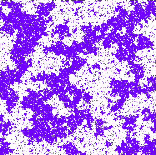
Do you notice something in this image? Anything sticking out?

Remarkably, it is not visible at first sight: the upper right quadrant of Figure 1 was replaced with a scaled-down and coarse-grained version of the original figure. Do you see it now? The pattern shown here exemplifies a system at its critical point, where the same kind of shapes can appear on all scales!
We will look at the Ising model to understand this phenomenon. The Ising model is the harmonic oscillator of statistical physics, in the sense that it serves as a foundational abstract model. The two dimensional Ising model is a minimal model that can show phase transitions at finite temperature. And importantly, it is still analytically solvable, as was shown by Onsager (1944). Here, we focus on considerations of scales of structures in the one and two-dimensional Ising model, which will lead us to a powerful technique applicable also beyond the Ising model: Renormalization. Finally, we will give a conceptual idea of how renormalization is leveraged to show the existence of a critical point at finite temperature in the 2D Ising model.
I wrote this as part of a handout for a seminar in statistical physics. I hope it offers a digestible resource to understand the interesting phenomenon of criticality and the power of renormalization.
Ising model
The Ising model is defined on a graph of "sites" \(i\), usually on a lattice. On every site, there is a scalar binary variable \(s_i = \pm 1\) and for configurations, the energy of the whole system is given by the Hamiltonian:
\[\mathcal{H} = \quad - J \sum_{<ij>} s_i s_j \quad - B \mu \sum_i s_i\]
The first term sums over nearest neighbor pairs of spins. For \(J>0\) alignment \(\uparrow\uparrow\) / \(\downarrow\downarrow\) of spins is favored in comparison to misalignment \(\uparrow\downarrow\) / \(\downarrow\uparrow\). We can nondimensionalize the equation with \(\beta = \frac {1}{k_b T}\) and absorb everything into new coupling constants \(K = \beta J\) and \(H = \beta B \mu\). \[ \beta \mathcal{H} = \quad - K \sum_{<ij>} s_i s_j \quad - H \sum_i s_i \label{hamiltonian} \tag{1}\]
Note, that the coupling is now temperature-dependent. High temperatures \(T\) correspond to low coupling \(H\) between neighboring spins.
Response to temperature
The Ising Hamiltonian Equation 1 describes the energy of any given configuration of the spins \(S_i\). Such a configuration is called a microstate. We imagine the spin system to be in contact with a heat reservoir, such that instead of the energy, the temperature is fixed.
To understand the interplay of temperature and energy in this so-called canonical ensemble, we turn our attention to the probability that the system may find itself with energy \(E\) for some temperature \(T\). The probability of microstates will follow a Bolzmann statistic \[\begin{aligned} p_i =& \frac 1 Z e^{-\beta E_i} \\ Z =& \sum_{\text{configurations}} e^{-\beta \mathcal{H}} \quad \quad \text{partition function} \end{aligned}\].
However, there are many different microstates that the Hamiltonian evaluates with \(E\). We call this number of microstates \(\Omega (E)\). Further, remember that the entropy is straightforwardly defined as the logarithm of said number \(S = k_B \ln \Omega\), such that \[\begin{aligned} p(E) &= \Omega(E) \cdot \frac 1 Z e^{-\beta E} \nonumber \\ &= \frac 1 Z e^{-\beta (E-TS)} = \frac 1 Z e^{-\beta F} \\ F &\coloneqq E-TS= - \frac 1 \beta \ln Z \quad. \end{aligned}\]We have defined the "free energy" \(F\) and observe, that the probability of a macrostate of energy \(E\) is both higher the lower its energy is and the higher its entropy is. The relative importance of these two trends is determined by temperature.
Figure 2 (a) is an example of pure energy minimization in the face of vanishing temperature. The other extreme, infinite temperature, where only entropy is relevant can be seen in Figure 2 (c). At the same time, the behavior can be explained solely by the temperature dependence of the coupling \(K=\beta J\): For \(T=0\) the coupling diverges, \(K\rightarrow \infty\), and consequently alignment dominates. If on the other hand due to the temperature diverging the coupling vanishes, \(K=0\), it only makes sense that even neighboring spins become independent.
Both extreme regimes would not change qualitatively under a zoom-out-and-coarse-grain operation. They would still show an aligned and a random configuration respectively. Between the extremes, however, there might be another such scale invariant temperature that separates the ordered from the unordered phase. Our next mission will be to show with some proof and hand waving, that there is such a critical point at finite temperature \(T_c\).

\(K\rightarrow\infty\)
\(K=K^*\)
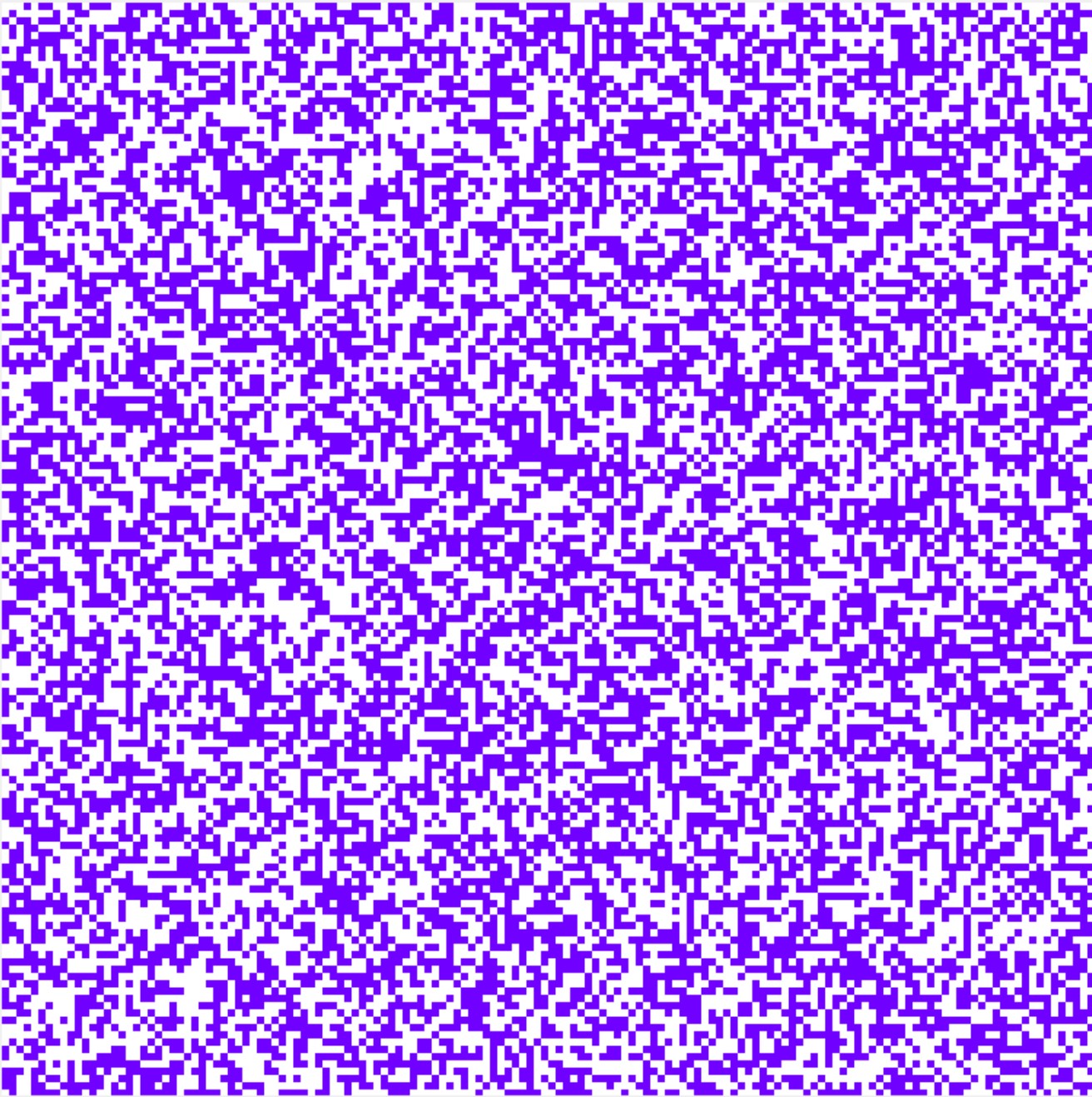
\(K=0\)
Ising chain
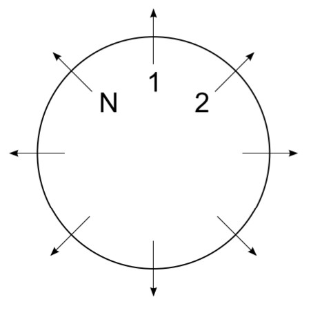
To quantify the size of fluctuations we should investigate the role of distance in the Ising model. To that end, we look at the correlation of spins at distance \(j\) and for now, restrict the considerations for simplicity to the one-dimensional Ising chain. Using the partition function of the Ising chain under periodic boundary conditions – the Ising ring, see Figure 3 – we will derive the expectation \(\langle s_i s_{i+j} \rangle\).
First, calculate the partition function for vanishing external field \(H\) by doing the summation over spin \(S_N\) explicitly. \[\begin{aligned} Z_N =& \sum_{\substack{\{ s_i \} \\ i=1...N}} e^{-\beta \mathcal{H}} \nonumber\\ =& \sum_{\substack{\{ s_i \} \\ i=1...N-1}} e^{-\beta \mathcal{H}} \left( e^{-K\cdot +1} + e^{-K \cdot -1}\right) \nonumber\\ =& \left(2 \cosh{(K)}\right) Z_{N-1} \quad . \end{aligned}\]This recursive equation can be iterated and we finally result with \[ Z_N = \left( 2 \cosh(K) \right)^N \quad . \tag{2}\]
To derive the expectation \(\langle s_i s_{i+j} \rangle\), we make use of a trick: Suppose every coupling is different, then Equation 2 becomes \(Z_N = \left( 2 \cosh(K_i) \right)^N\). With this, we can write
\[\begin{aligned} \langle s_i s_{i+j} \rangle &= \sum_{\substack{\{ s_i \} \\ i=1...N-1}} s_i s_{i+j} e^{-\beta \mathcal{H}}\\ &= \sum_{\substack{\{ s_i \} \\ i=1...N-1}} (s_i s_{i+1})(s_{i+1} s_{i+2}) ... (s_{i+j-1} s_{i+j}) e^{-\beta \mathcal{H}} \nonumber \\ &= \partial_{K_i} ... \partial_{K_{i+j-1}} \ln Z_N\\ \end{aligned}\]Here we have introduced \(s_{k}^2\) for \(k\) between \(i\) and \(j\) which will always be \(1\) in the first step. Then, the spin pairs correspond to derivatives for the couplings \(K_i\). Ultimately, the derivative is \[ \langle s_i s_{i+j} \rangle = \left( \tanh K \right)^j = e^{-j/\xi} \quad \quad \xi = - \frac{1}{\ln \left( \tanh K \right)} \tag{3}\]
since \(\partial_x \cosh(x) = \sinh(x)\) and \(\frac{\sinh(x)}{\cosh(x)} = \tanh (x)\).
In the end, we don’t distinguish couplings anymore, so \(K_i = K\). The decay of correlation follows an exponential function (Equation 3) for which we define the characteristic length scale \(\xi = - \frac{1}{\ln \left( \tanh K \right)}\).
Renormalization
Depending on temperature and coupling microstates will have "islands" of alignment that differ in size. The correlation length is a natural scale for the size of structures, since information decays by \(1/e\) for every \(\xi\). Turned around, a coupling/temperature that leads to scale-invariant probability distribution with finite-sized islands must give rise to islands of any other scale and thus must have a diverging correlation length \(\xi\).
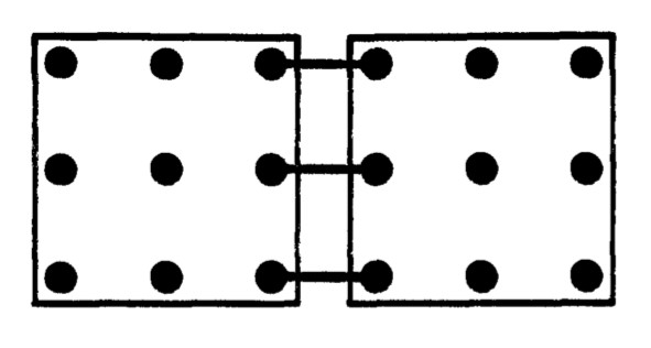
To search for the critical point (Figure 2 (b)) we define a zooming-out-and-coarse-grain operation – renormalization. One example is the Block renormalization, shown in Figure 4 (a) for two dimensions.
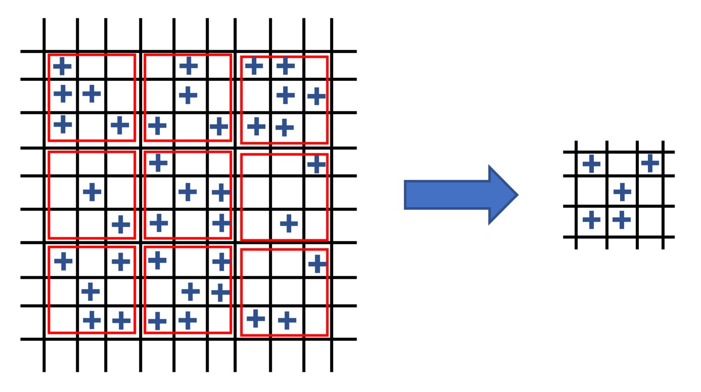
We can think of the resulting system as a modified one and hope that its Hamiltonian \(\mathcal{H'}\) is of similar form. In general, applying such an operation to the Ising model, which has only nearest neighbor interactions, will introduce infinitely more couplings between the resulting coarse-grained spins \(s_i'\). This can be appreciated when referencing Figure 4 (b). By summing over the corner spin effectively a diagonal interaction is created. So we understand, that \(\mathcal{H'}\) will not be exactly of the form of \(\mathcal{H}\), but if we find a sufficiently close approximation of \(\mathcal{H'}\), we can iterate the renormalization operation \(\mathcal{R}\).
A fixpoint of \(\mathcal{R}\) then corresponds to a temperature/coupling that is scale invariant. Thus, we will search for such a fixed point in the following.
\(\mathcal{R}\) for the chain
We will explicitly derive the flow of the coupling under \(\mathcal{R}\) for the 1D Ising chain first, before turning to the 2D system again.
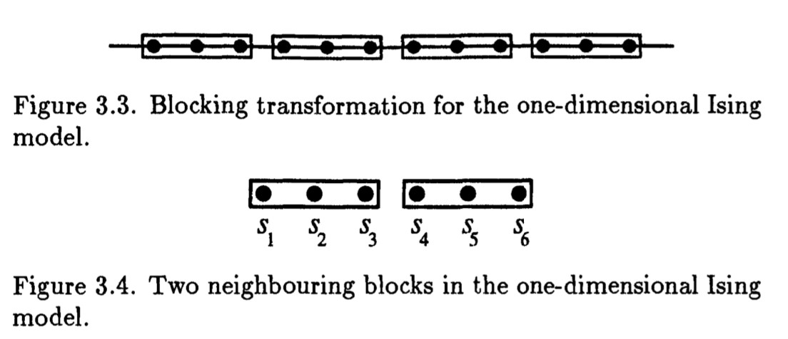
Consider the block renormalization scheme for the 1D case shown in Figure 5. We can explicitly sum over the degrees of freedom that are lost by applying \(\mathcal{R}\).
\[\sum_{s_3, s_4} e^{K s'_1 s_3 }e^{K s_3 s_4 }e^{K s_4 s'_2 } = 4 (\cosh K)^3 (1+(\tanh K )^3 s'_1 s'_2 )\]
The result has a constant term, that we can safely ignore since energy is only defined up to a constant anyway. But importantly we find also a product \(s'_1 s'_2\) of the new spins, which recovers the nearest neighbor interaction. The factor in front of it can be identified as the new coupling \(K'\).
We have derived the flow of the coupling.
\[ K' = \tanh^{-1}\left( (\tanh K )^3 \right) \]
An equivalent decluttered form is obtained by defining \(k=\tanh K\) and \(k'=\tanh K'\). \[ k' = k^3 \]
Application of the renormalization operator \(\mathcal{R}\) leaves the structure of the Hamiltonian intact, such that we can repeat it iteratively. After each iteration, we still have a chain of spins governed by a Hamilton with nearest-neighbor interaction. But with each iteration, the coupling changes according to the iterative map. If and only if the map has a fixed point at that coupling, the Hamiltonian and the resulting pattern distribution is the same for all zoom levels!
We can conveniently inspect the iterative map for fixed points by plotting them.
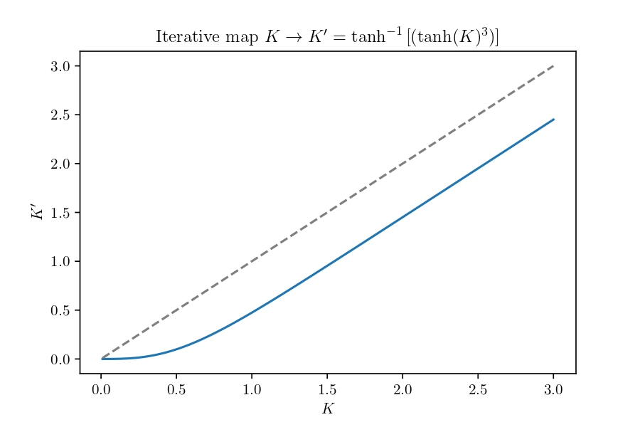
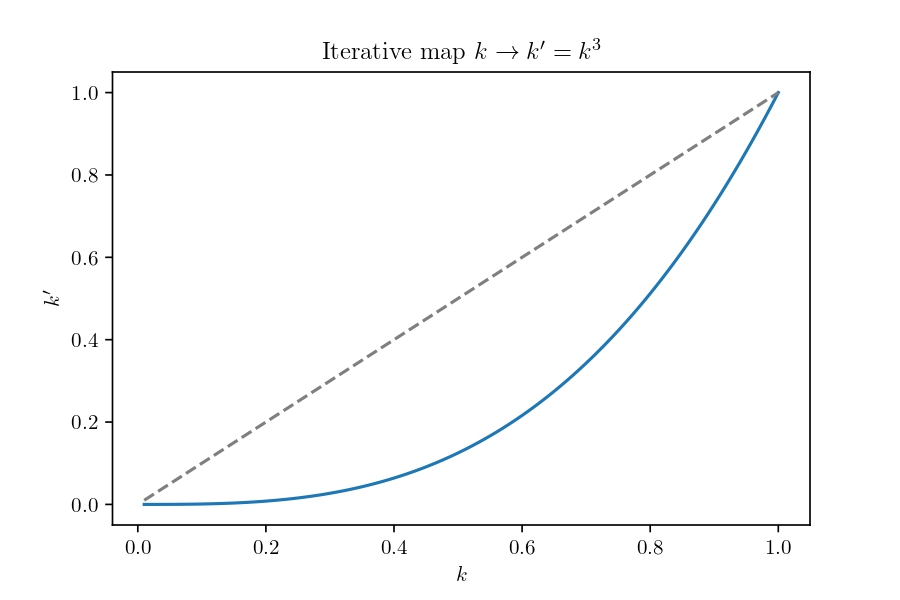
An intersection of the map with the identity (diagonal) signifies a fixed point. We find an unstable fixed point at \(k=1\), i.e. \(K\rightarrow\inf\), and a stable fixed point at \(K=k=0\). This means the Ising chain has no critical state at a finite coupling/temperature. Rather, zooming out reduces the coupling until it hits zero. Zero coupling, i.e. infinite temperature corresponds to a random unordered state.
Sanity check: correlation length
How does the correlation length \(\xi(K)\) transform under renormalization? Since zooming out effectively increases the distance between spins by a factor and it solely depends on the coupling, we can write
\[\begin{align*} \xi(\tanh K') &= b^{-1} \xi(\tanh K) \\ &= \xi((\tanh K)^3) \end{align*}\] \[\begin{equation} \Rightarrow \xi = \frac{\text{const.}}{\ln \tanh K} \end{equation}\]
Note, that we have recovered the result that we have derived rigorously before in Equation 3.
\(\mathcal{R}\) for the 2D model
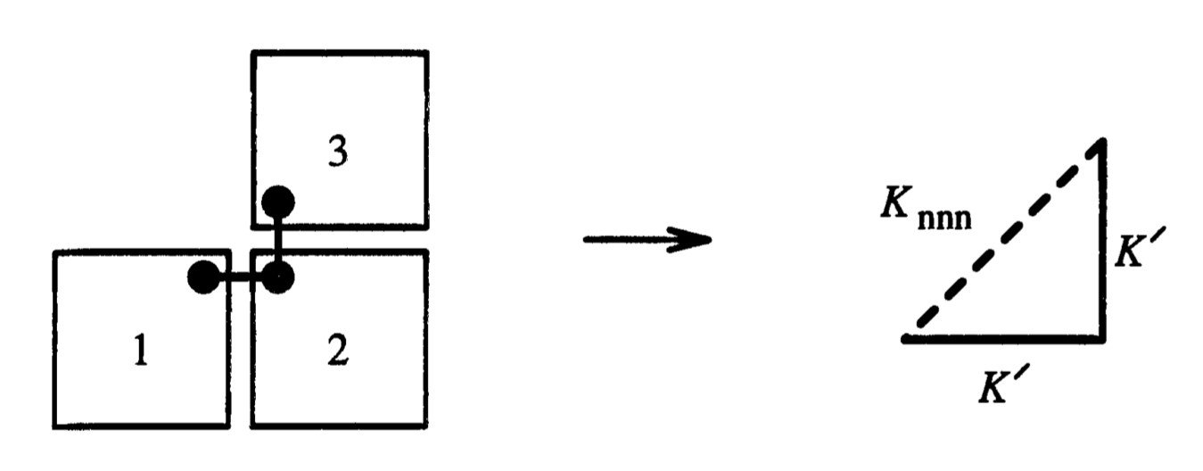
As can be seen in Figure 7, for the chosen block renormalization scheme three old couplings \(K\) are replaced with just one coupling \(K'\). We can compare that in the Ising chain the flow of high \(K\) (cf. ) can be written as \(K' \sim K - const.\)
\[\begin{equation} K' \sim 3K - const. \end{equation}\]
Consequently, the coupling flow is steeper than the identity and must cross it eventually. On the intersection, we have an unstable fixpoint at finite temperature.
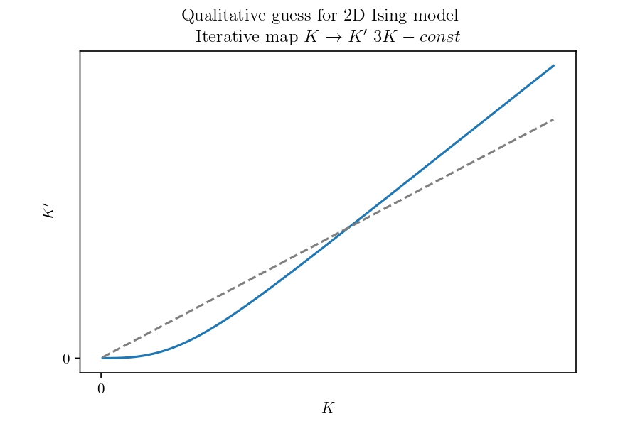
This qualitative argument proves the existence of a finite temperature phase transition – a critical point where the correlation length diverges and the scale of everything is arbitrarily small or big. To find the actual temperature where the phase transition happens, you need to explicitly find \(\mathcal R\), the corresponding coupling flow, and its fixed point. For this work and more broadly developing renormalization group theory, Kenneth G. Wilson was awarded the Nobel Prize in Physics in 1982.