n = 128
m = n^2
@time zeros(m,m);
1.633549 seconds (163 allocations: 2.000 GiB, 0.74% gc time, 0.36% compilation time)I share some performance benchmarks for different algorithms of (generalized) matrix inversion.
A current project requires me to do one costly operation repeatedly for different input data. After an initial implementation it became clear each single repetition takes around a minute. Since I need thousands of repetitions and will inevitably have to repeat the whole analysis multiple times, this was a situation where optimization really matters.
To avoid letting a computer run for \(n\cdot10^4\) minutes (about \(n\cdot 7\) days), we need to be faster.
There are many possible reasons to try and find the generalized inverse of a large matrix and here my use case does not really matter outside of this “motivation” box. Anyways, my situation is:
Experts hand-crafted a procedure to extract structural information out of pattern data (see Schnörr and Schnörr 2021). This involves constructing a graph from an image of the pattern (say with \(128\times 128\) pixels). Then, to calculate the resistance distance between vertices of the graph (corresponding to pixels in the image) we need the generalized inverse of the Laplacian matrix 1 of said graph (see Klein and Randić 1993).
You might know the adjacency matrix that describes the edges of a graph. The Laplacian is the negative adjacency matrix but with the row sum of the adjacency matrix on its diagonal. Because of this construction, importantly, the rows (and columns) of the Laplacian sum up to 0.
My project involves studying how these expert-crafted statistics for pattern quantification can be used in conjuction with machine-learnt statistics. Finally, the goal is to solve the inverse problem of pattern formation, that is, which system parameters of the pattern forming model are likely to have resulted in this or that pattern I might have observed.
This graph Laplacian is what we call \(A\) in the following to stay abstract. Graphs are ubiquitous and getting distances quickly might matter to other people and problems as well. Refer to Shuman et al. (2013) for a well-written overview.
Find the fastest way to compute the generalized inverse \(G\) of a matrix \(A \in \mathbb R ^{m\times m}\) which is
Lastly, \(A\) is very large, since \(m=16384 = n^2\) with \(n=128\) in my specific case.
\(G\) is called a generalized inverse (g-inverse) to \(A\) if and only if
\[ AGA = A \tag{1}\]
and such a g-inverse exists for arbitrary matrices. For invertible matrices the g-inverse is unique and it is the regular inverse \(A^{-1}\) (defined by \(A A^{-1} = \mathbb 1\)).
Most libraries for fast numerical computation have an implementation of the so-called Moore-Penrose pseudo-inverse, a specific g-inverse. The algorithm is based on singular value decomposition and can be applied to arbitrary matrices to get a g-inverse. This means it would also compute the regular inverse if given an invertible matrix, just less efficiently. If you know \(A\) to be invertible, it is quicker to e.g. use a LU decomposition.
The discussed algorithms are available in numpy and scipy; use [numpy, scipy].linalg.pinv(A) for the pseudo-inverse and [numpy, scipy].linalg.inv(A) for the regular inverse.
Since our \(A\) is not invertible, we are currently stuck with using pinv.
The matrix is so large, that we should imediately think about whether we can use that most of the elements are zero (sparsity). Let’s quickly look at the memory and time cost of simply allocating a matrix like this without exploiting its sparsity.
n = 128
m = n^2
@time zeros(m,m); 1.633549 seconds (163 allocations: 2.000 GiB, 0.74% gc time, 0.36% compilation time)That is a lot! If the task was just to, for example, multiply two matrices of such size, it would be hugely beneficial to just keep track of the non-zero elements.
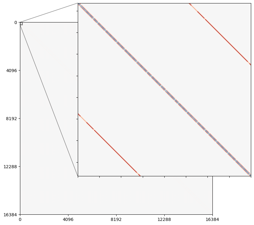
It turns out however, that there is no algorithm to exploit matrix sparsity for inversion, since (in general) the (g-)inverse of a sparse matrix is dense. The exception is if you can find a block-diagonal form of \(A\), the (g-)inverse will also be block-diagonal and you can invert the blocks individually.
Since our matrix \(A\) is banded, there are no disconnected components of rows, and consequently no way to permute rows and columns to form disconnected blocks and thus ultimately we cannot exploit the sparsity.
So are we stuck with the Moore-Penrose pseudo-inverse? No, there are more matrix properties to exploit!
It turns out that we can use that each row of \(A\) sums up to 0. Theorem 1 lets us map the search for a g-inverse of a matrix \(A\) for which the regular inverse does not exist on the regular inverse of a related matrix.
Theorem 1 (Plus 1 trick) Let \(A \in \mathbb{R}^{m \times m}\) be a matrix with zero row sum. Let \(\mathbf{1}\) be the \(m \times m\) matrix where every entry is 1. Then, if the inverse of \(B=A+\mathbf{1}\) exists, it is also a g-inverse of \(A\).
To see why this holds, note that since \(B = A + \mathbf{1}\), every row and column of \(B\) sums to \(m\), and the rows of \(B^{-1}\) sum to \(\frac{1}{m}\), implying \[ B^{-1} \mathbf{1} = \frac{1}{m} \mathbf{1}\,. \] Thus, the second term becomes \[ A \frac{1}{m} \mathbf{1} = 0\,, \] because \(A\) annihilates constant vectors (i.e., \(A \mathbf{1}_m = 0\) by assumption, since the row and column sums of \(A\) are zero). Therefore, we conclude \[ A B^{-1} \mathbf{1} = 0\,. \] This simplifies the original equation to \[ A = A B^{-1} A \] which completes the proof.
Since \(A\) is symmetric, diagonally-dominant and has zero row sums, we can apply Theorem 2 to see that the requirements of the Cholesky decomposition are met for \(A + \mathbf{1}\). 2
Since the Cholesky decomposition is about twice as fast as the LU decomposition, the “plus 1 trick” from Theorem 1 can be sped up further.
Theorem 2 (Positive semidefiniteness) Let \(A\) be a symmetric, diagonally dominant matrix with zero row and column sums. Let \(\mathbf{1}\) be the \(m \times m\) matrix where every entry is 1. Then the matrix \(B = A + \mathbf{1}\) is positive semidefinite.
Since \(A\) is symmetric and has zero row and column sums, \(A \mathbf{v} = 0\) for \(\mathbf{v} = (1, 1, \ldots, 1)^T\). This means 0 is an eigenvalue of \(A\) with eigenvector \(\mathbf{v}\).
The matrix \(\mathbf{1}\) has eigenvalues \(m\) (with multiplicity 1) and \(0\) (with multiplicity \(m-1\)). The eigenvector corresponding to \(m\) is \(\mathbf{v}\).
For the eigenvector \(\mathbf{v}\): \[ B \mathbf{v} = (A + \mathbf{1})\mathbf{v} = A \mathbf{v} + \mathbf{1} \mathbf{v} = 0 + m\mathbf{v} = m\mathbf{v} \] So, \(m\) is an eigenvalue of \(B\).
For any vector \(\mathbf{u}\) orthogonal to \(\mathbf{v}\) (i.e., \(\mathbf{v}^T \mathbf{u} = 0\)): \[ B \mathbf{u} = (A + \mathbf{1})\mathbf{u} = A \mathbf{u} + \mathbf{1} \mathbf{u} = A \mathbf{u} + 0 = A \mathbf{u} \] Since \(A\) is diagonally dominant and symmetric with zero row sums, it is positive semidefinite. Therefore, \(\mathbf{u}^T A \mathbf{u} \geq 0\).
Since eigenvectors of symmetric matrices like \(B\) are orthogonal, we have considered all eigenvalues of \(B\) and showed they are non-negative, proving that \(B = A + \mathbf{1}\) is positive semidefinite.
For speed comparisons we use the matrices we actually want to g-invert. In this specific case we construct a graph from reaction diffusion patterns and calculate its Laplacian, Tip 1.
using Pkg
Pkg.activate("."; io=devnull)
using LinearAlgebra
using LinearAlgebra: BlasReal, BlasFloat
using BenchmarkTools
using Plots
using BenchmarkPlots
import StatsPlots
using Measures
using PyCall
@pyimport pickle

function mypickle(filename, obj)
    out = open(filename,"w")
    pickle.dump(obj, out)
    close(out)
end

function myunpickle(filename)
    r = nothing
    @pywith pybuiltin("open")(filename,"rb") as f begin
        r = pickle.load(f)
    end
    return r
end

import_dict = myunpickle("data/sim_long_preprocessed_slice.pkl")
Dict{Any, Any} with 2 entries:
"parameters" => [0.0608592 2.59401 … 0.5 1.0; 0.0933432 2.58813 … 0.5 1.0; … …
"patterns" => [0.394308 0.342241 … 0.273087 0.381393; 0.380113 0.3699 … 0.3…test_pattern = import_dict["patterns"][1,:,:]
heatmap(test_pattern, cmap=:seaborn_icefire_gradient, aspect_ratio=:equal, xlim=(1,size(test_pattern)[1]), ylim=(1,size(test_pattern)[2]), size=(300,300), margin=3mm)
The weighted adjacency matrix is created by simply looping over the patterns pixels and choosing weights of neighboring pixels according to the pattern “color”.
function get_adj_matrix(pattern, ε=0.003)
    @assert size(pattern, 1) == size(pattern, 2)
    graph_res = size(pattern, 1)
    m = graph_res^2
    adj_matrix = zeros(Float64, m, m)
    u_mean = mean(pattern)

    for i in 1:m
        neighbor_js = [i - 1, i + 1, i - graph_res, i + graph_res]
        neighbor_js = mod1.(neighbor_js, m)# .+ 1

        for j in neighbor_js
            u_vi = pattern[mod1(i, graph_res), div(i - 1, graph_res) + 1]
            u_vj = pattern[mod1(j, graph_res), div(j - 1, graph_res) + 1]
            vi_high = u_vi > u_mean
            vj_high = u_vj > u_mean
            adj_matrix[i, j] = vi_high == vj_high ? 1.0 : ε
        end
    end

    return adj_matrix
end

function prepare_graph_laplacian_matrix(pattern, ε)
    graph_res = size(pattern, 1)
    m = graph_res^2

    adj_matrix = get_adj_matrix(pattern, ε)
    graph_laplacian = Diagonal(adj_matrix * ones(m)) - adj_matrix
    return graph_laplacian
end

ε = 0.003
laplacian = prepare_graph_laplacian_matrix(test_pattern, ε)
16384×16384 Matrix{Float64}:
4.0 -1.0 0.0 0.0 0.0 … 0.0 0.0 0.0 0.0 -1.0
-1.0 4.0 -1.0 0.0 0.0 0.0 0.0 0.0 0.0 0.0
0.0 -1.0 2.006 -0.003 0.0 0.0 0.0 0.0 0.0 0.0
0.0 0.0 -0.003 2.006 -1.0 0.0 0.0 0.0 0.0 0.0
0.0 0.0 0.0 -1.0 3.003 0.0 0.0 0.0 0.0 0.0
0.0 0.0 0.0 0.0 -1.0 … 0.0 0.0 0.0 0.0 0.0
0.0 0.0 0.0 0.0 0.0 0.0 0.0 0.0 0.0 0.0
0.0 0.0 0.0 0.0 0.0 0.0 0.0 0.0 0.0 0.0
0.0 0.0 0.0 0.0 0.0 0.0 0.0 0.0 0.0 0.0
0.0 0.0 0.0 0.0 0.0 0.0 0.0 0.0 0.0 0.0
0.0 0.0 0.0 0.0 0.0 … 0.0 0.0 0.0 0.0 0.0
0.0 0.0 0.0 0.0 0.0 0.0 0.0 0.0 0.0 0.0
0.0 0.0 0.0 0.0 0.0 0.0 0.0 0.0 0.0 0.0
⋮ ⋱ ⋮
0.0 0.0 0.0 0.0 0.0 0.0 0.0 0.0 0.0 0.0
0.0 0.0 0.0 0.0 0.0 0.0 0.0 0.0 0.0 0.0
0.0 0.0 0.0 0.0 0.0 0.0 0.0 0.0 0.0 0.0
0.0 0.0 0.0 0.0 0.0 … 0.0 0.0 0.0 0.0 0.0
0.0 0.0 0.0 0.0 0.0 0.0 0.0 0.0 0.0 0.0
0.0 0.0 0.0 0.0 0.0 0.0 0.0 0.0 0.0 0.0
0.0 0.0 0.0 0.0 0.0 -1.0 0.0 0.0 0.0 0.0
0.0 0.0 0.0 0.0 0.0 4.0 -1.0 0.0 0.0 0.0
0.0 0.0 0.0 0.0 0.0 … -1.0 4.0 -1.0 0.0 0.0
0.0 0.0 0.0 0.0 0.0 0.0 -1.0 3.003 -0.003 0.0
0.0 0.0 0.0 0.0 0.0 0.0 0.0 -0.003 3.003 -1.0
-1.0 0.0 0.0 0.0 0.0 0.0 0.0 0.0 -1.0 4.0Let us have a function to check if \(G\) is actually the g-inverse to \(A\).
function check_g_inverse(A, G)
    return isapprox(A * G * A, A)
end;
function randposdef(N)
A = randn(N, N)
return Symmetric(A * A' + I)
end
A = randposdef(3)
B = randposdef(3)3×3 Symmetric{Float64, Matrix{Float64}}:
1.42807 -0.703668 -0.128767
-0.703668 6.37562 -4.00037
-0.128767 -4.00037 5.29409The following should pass as the inverse of a full rank matrix is also its g-inverse.
@assert check_g_inverse(A,inv(A)) "check failed: not a g-inverse!"The following should fail as the matrices do not fit each other.
# when uncommenting the next line, my document does not compile anymore. Just as it should.
# @assert check_g_inverse(A,inv(B)) "check failed: not a g-inverse!"
Great! Everything as expected.
pinv(A) vs. inv(ones(m,m) + A)Now we calculate the g-inverse of the same test matrices with different algorithms accross different matrix sizes \(m\).
We are going to compare the Moore-Penrose pseudo inverse with the above described “Plus 1 trick” to which we can apply the implementations of for regular matrix inversion. In the Python-world, we are looking at both numpy and scipy. Both additionally have a pseudo-inverse implementation that can exploit a matrix being Hermitian. Since our \(A\) is symmetric and real, this algo is appliable for us and we include it in the comparison.
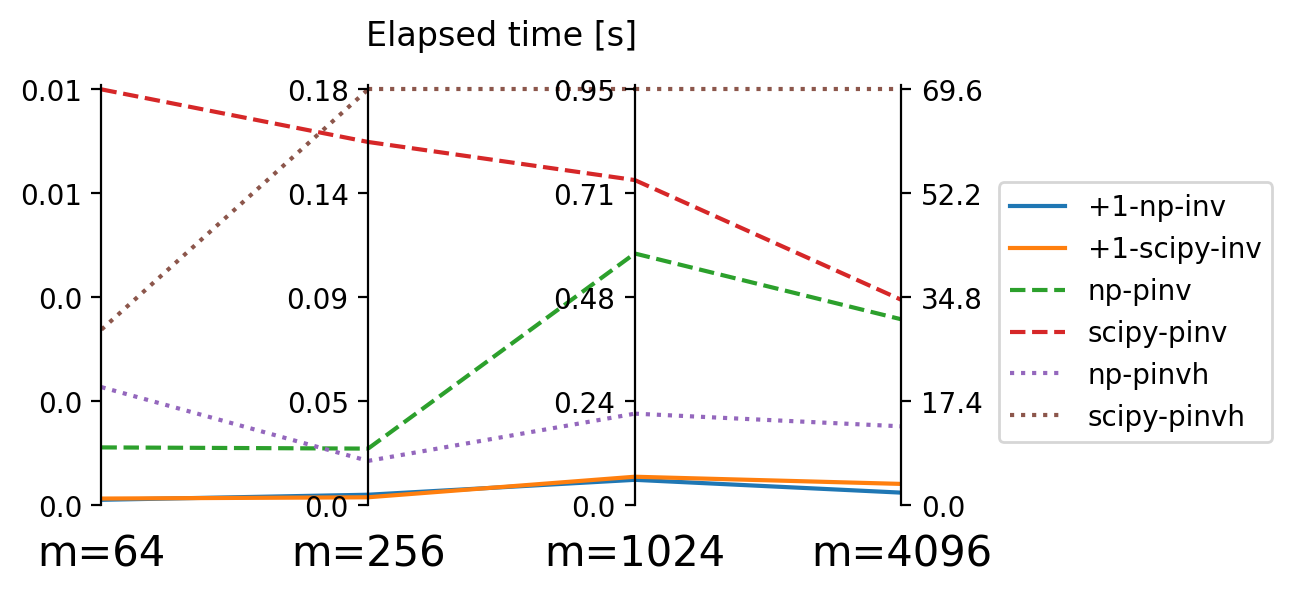
numpy and scipy accross matrix size \(m\).
numpy vs. scipy does not play a big role, with the exception of the Hermitian implementation where numpy outcompetes scipy substantially Figure 3.
But this effect is dominated by the “plus 1 trick” which allows us to be apparently much faster than relying on Moore-Penrose pseudo-inverse algorithms. In fact, elapsed time for the latter explodes so much for large matrix size \(m\) that we exclude them for benchmarks on \(m>4000\) shown in Figure 4.
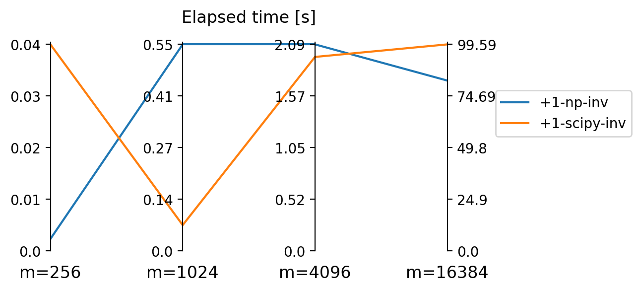
numpy and scipy for very high matrix size \(m\).
Only thanks to danielwe’s insightful post on the Julia forum, I heard about the undocumented method LinearAlgebra.inv!(cholesky!(A)). It is exactly what we need. First, it saves time by doing the computation in-place, avoiding superfluous allocations that, as we saw in Section 2.1, can waste a significant amount of time. Second, it exploits the Cholesky decomposition which should speed it up roughly two-fold.
function inv!(A)
    A = LinearAlgebra.inv!(cholesky!(A))
end
inv! (generic function with 1 method)We can further use the fact that \(A\) is symmetric and use the lower triangle of the matrix as a workspace to save allocations. The below implementation uses the LAPACK API directly to achieve this and thus should be a bit faster than the above.
function invlapack!(A::Union{Symmetric{<:BlasReal},Hermitian{<:BlasFloat}})
    _, info = LAPACK.potrf!(A.uplo, A.data)
    (info == 0) || throw(PosDefException(info))
    LAPACK.potri!(A.uplo, A.data)
    return A
end
invlapack! (generic function with 1 method)Finally, we need a function that adds 1 before applying inv! or invlapack! and does all of this in-place to save allocations. We generate this function with a metafunction add_one_then_fun(fun).
function add_one_then_fun(fun)
    funname = string(fun)
    return eval(:(@eval function ($(Symbol("add_one_then_$funname")))(A)
        A += ones(size(A))
        A = $fun(Symmetric(A))
    end))
end
add_one_then_fun(invlapack!)
add_one_then_invlapack! (generic function with 1 method)function choose_appropriate_time(A)
if size(A)[1] <= 32^2
seconds = 30
elseif size(A)[1] <= 64^2
seconds = 60
else
seconds = 240
end
return seconds
end;We set up a group of benchmarks for different sizes of \(A\) with pseudo-inverse (pinv) and regular inverse of \(A + \mathbf 1\) (add_one_then_fun(inv!) and add_one_then_fun(invlapack!)) with the two fast inverse implementations that use a Cholesky decomposition.
suite = BenchmarkGroup()
for pattern_size in (8, 16, 32, 64, 128)
    test_pattern = import_dict["patterns"][1,1:pattern_size, 1:pattern_size]
    laplacian = prepare_graph_laplacian_matrix(test_pattern, ε)

    A = Symmetric(laplacian)
    seconds = choose_appropriate_time(A)

    for f in (pinv, add_one_then_fun(inv!), add_one_then_fun(invlapack!))
        if pattern_size > 16 && f == pinv  # skip slow pseudo-inverse computation for large A
           continue
        end
        @assert check_g_inverse(A, f(copy(A))) "" * string(f) * "(copy(A)) is not a g-inverse of A"
        suite[pattern_size^2][Symbol(f)] = @benchmarkable $(f)($A) evals=1 seconds=seconds
    end
end
suite
5-element BenchmarkTools.BenchmarkGroup:
tags: []
64 => 3-element BenchmarkTools.BenchmarkGroup:
tags: []
"add_one_then_invlapack!" => Benchmark(evals=1, seconds=30.0, samples=10000)
"add_one_then_inv!" => Benchmark(evals=1, seconds=30.0, samples=10000)
"pinv" => Benchmark(evals=1, seconds=30.0, samples=10000)
1024 => 2-element BenchmarkTools.BenchmarkGroup:
tags: []
"add_one_then_invlapack!" => Benchmark(evals=1, seconds=30.0, samples=10000)
"add_one_then_inv!" => Benchmark(evals=1, seconds=30.0, samples=10000)
4096 => 2-element BenchmarkTools.BenchmarkGroup:
tags: []
"add_one_then_invlapack!" => Benchmark(evals=1, seconds=60.0, samples=10000)
"add_one_then_inv!" => Benchmark(evals=1, seconds=60.0, samples=10000)
16384 => 2-element BenchmarkTools.BenchmarkGroup:
tags: []
"add_one_then_invlapack!" => Benchmark(evals=1, seconds=240.0, samples=10000)
"add_one_then_inv!" => Benchmark(evals=1, seconds=240.0, samples=10000)
256 => 3-element BenchmarkTools.BenchmarkGroup:
tags: []
"add_one_then_invlapack!" => Benchmark(evals=1, seconds=30.0, samples=10000)
"add_one_then_inv!" => Benchmark(evals=1, seconds=30.0, samples=10000)
"pinv" => Benchmark(evals=1, seconds=30.0, samples=10000)The whole benchmark suite can be run simultaneously.
results = run(suite, verbose = false)5-element BenchmarkTools.BenchmarkGroup:
tags: []
64 => 3-element BenchmarkTools.BenchmarkGroup:
tags: []
"add_one_then_invlapack!" => Trial(80.301 μs)
"add_one_then_inv!" => Trial(56.977 μs)
"pinv" => Trial(510.179 μs)
1024 => 2-element BenchmarkTools.BenchmarkGroup:
tags: []
"add_one_then_invlapack!" => Trial(15.356 ms)
"add_one_then_inv!" => Trial(17.253 ms)
4096 => 2-element BenchmarkTools.BenchmarkGroup:
tags: []
"add_one_then_invlapack!" => Trial(826.550 ms)
"add_one_then_inv!" => Trial(864.252 ms)
16384 => 2-element BenchmarkTools.BenchmarkGroup:
tags: []
"add_one_then_invlapack!" => Trial(39.769 s)
"add_one_then_inv!" => Trial(40.473 s)
256 => 3-element BenchmarkTools.BenchmarkGroup:
tags: []
"add_one_then_invlapack!" => Trial(683.294 μs)
"add_one_then_inv!" => Trial(674.657 μs)
"pinv" => Trial(8.485 ms)For each matrix size \(m\) we can compare the run times amongst the different g-inverse implementations:
plots = Dict()
for key in keys(results)
    plots[key] = StatsPlots.plot(results[key], title="time for g-inverse of \$ A \\in \\mathbb{R}^{m \\times m} \$ with \$m=$(string(key))\$")  #; yscale=:log10)
end
l = @layout (5, 1)
plot(plots[64], plots[256], plots[1024], plots[4096], plots[16384], layout = l, size=(600,1000), left_margin=10mm)
Like we saw previously in the Python benchmark computations, the pinv pseudo-inverse is considerably slower. As expected the LAPACK implementation of the Cholesky decomposed matrix from the “plus 1 trick” is the fastest.
This represents an additional 3-fold speed improvement compared to the best Python implementation.
results[16384][add_one_then_inv!]BenchmarkTools.Trial: 5 samples with 1 evaluation. Range (min … max): 40.473 s … 47.605 s ┊ GC (min … max): 0.85% … 0.85% Time (median): 45.019 s ┊ GC (median): 0.90% Time (mean ± σ): 44.744 s ± 2.792 s ┊ GC (mean ± σ): 0.95% ± 0.42% █ █ █ █ █ █▁▁▁▁▁▁▁▁▁▁▁▁▁▁▁▁▁▁▁▁▁▁▁▁▁▁█▁▁▁▁▁▁▁▁█▁▁▁▁▁▁▁▁▁▁▁▁▁█▁▁▁▁▁█ ▁ 40.5 s Histogram: frequency by time 47.6 s < Memory estimate: 4.00 GiB, allocs estimate: 4.
results[16384][add_one_then_invlapack!]BenchmarkTools.Trial: 5 samples with 1 evaluation. Range (min … max): 39.769 s … 47.624 s ┊ GC (min … max): 1.10% … 1.78% Time (median): 42.209 s ┊ GC (median): 0.84% Time (mean ± σ): 43.256 s ± 3.152 s ┊ GC (mean ± σ): 1.01% ± 0.49% █ █ █ █ █ █▁▁▁▁▁▁▁▁▁▁█▁▁▁▁▁█▁▁▁▁▁▁▁▁▁▁▁▁▁▁▁▁▁▁▁▁▁█▁▁▁▁▁▁▁▁▁▁▁▁▁▁▁▁█ ▁ 39.8 s Histogram: frequency by time 47.6 s < Memory estimate: 4.00 GiB, allocs estimate: 4.
We systematically exploited the matrix properties and were awarded a speed-up of several magnitudes.
For a \(m \times m\)-matrix with \(m=16384\) the computation of a pseudo-inverse by conventional methods was prohibitively expansive. In 4-fold reduced matrices, \(m=4096\), we found a 35x faster implementation by adding ones to the matrix before inverting with a conventional LU decomposition.
Implementing this in Julia and using a (optimized) Cholesky decomposition devided the time requirement by another factor of 3.
The winner is:
add_one_then_invlapack!(A)This function takes 26 seconds to compute the g-inverse. Without the optimizations we would have waited over half an hour.
To compute resistance distances matrices for 4000 different patterns (I need to do this), we would have waited from 36 days (conservative estimate) to 130 days (more likely).
This comes down to 1.2 days with the optimizations.
For the Laplacian matrix of a graph refer to this intuitive explanation which compresses a longer publication about it.↩︎
Beware the notation here. This is not the identity matrix. It is a matrix with every element being a 1.↩︎